import geopandas
import pandasExploring Change Over Time
30 minutes
![]()
In this session, we will explore how embeddings can be used to analyse change over time in a given area. The premise is (relatively) simple: if an embedding captures the content of an image in a series of numbers, we can use the changes in these numbers between the embeddings of an area across two periods of time to evaluate how much the area has changed.
We structure the analysis in four stages:
- Compute distances over time
- Explore change through these distances
- Mapping change
- Identifying types of change
Setup
For this session, we will be using the 2020 and 2024 versions of our embeddings for London LSOA’s data product. If you have not downloaded it yet, have a look at the data section in Materials.
We’ll go ahead and read the file with geometries and the embeddings (and set the area code as indices):
emb20 = geopandas.read_file('uk_lsoa_london_embeds_2020.geojson').set_index('data_zone_code')
emb24 = geopandas.read_file('uk_lsoa_london_embeds_2024.geojson').set_index('data_zone_code')
ERROR 1: PROJ: proj_create_from_database: Open of /opt/conda/envs/gds/share/proj failedCompute distances across periods
To compute distances, we rely on the same ideas we discussed in the previous session. We will use cosine distances but to what we apply them will change. Instead of computing distances between the embeddings of different areas, we will calculate them for the same area across two different periods. For this, paired_cosine_distances in Scikit-learn is a good fit:
from sklearn.metrics.pairwise import paired_cosine_distancesThis will calculate the distance, row-wise, for the embeddings of each area between 2020 and 2024:
distances = paired_cosine_distances(
    emb20.loc[:, 'A00_mean':'A63_mean'].values,
    emb24.loc[:, 'A00_mean':'A63_mean'].values
)
distances = pandas.Series(distances, index=emb20.index)
Explore change
Once we have the distance calculated, we can have a look:
Code
import matplotlib.pyplot as plt

p95 = distances.quantile(0.95)
p99 = distances.quantile(0.99)

fig, ax = plt.subplots(figsize=(9, 3))
n, bins, patches = ax.hist(distances, bins=150)

ax.axvspan(p95, distances.max(), color='green', alpha=0.3, label='Top 5%')
ax.axvspan(p99, distances.max(), color='red', alpha=0.3, label='Top 1%')

ax.set_title("Change 2020-24")

ax.legend()
plt.show()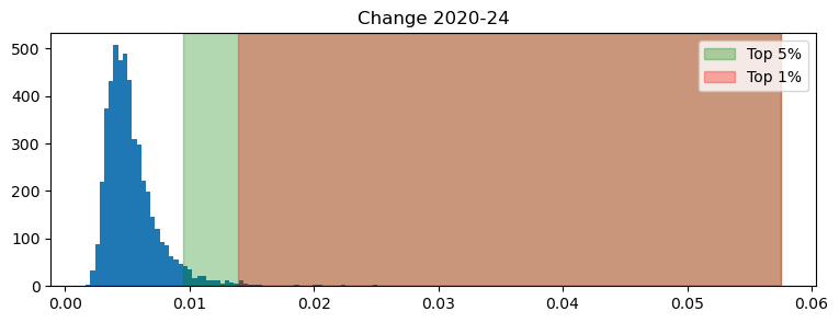
Note how heavily skewed the distribution is. This has a direct interpretation in meaningful terms: while most areas have not experienced much change, a few (particularly the top 1%), has seen significant differences recorded in the embedding numbers.
Identify changing areas
Knowing some areas have changed is all good and well but, as geographers, the next question this raises is obvious: where are such areas? In other words, what is the geography of change? Exploring this with our setup is fairly straight foward. For example, here’re the areas in the top 5% of the plot above:
Areas between top 5% and 1%:
Code
top5 = distances[distances > p95].index
(
    emb20
    .loc[top5, ['geometry']]
    .explore()
)
Make this Notebook Trusted to load map: File -> Trust Notebook
TipHome assignment
Make a similar map for the top 1%. Where are the areas that really have changed?
Becoming more like…
We now take everything we’ve learned in both sessions and apply to the following question: can we use embeddings to identify areas that have become more like other areas? For example, which area became more like Hyde Park in the period between 2020 and 2024?
To answer this question, we need to unpack it into the building blocks of an answer. To find out which LSOA changed more towards the character of Hyde Park, we can follow these steps:
- Calculate the distance between every area and Hyde Park in 2020
- Calculate the distance between every area and Hyde Park in 2024
- Obtain the difference between both distances, for every LSOA
- Pick the largest difference
Let’s get to work. To calculate these distances, we rely on a slightly different version of what we used above. cosine_distances will give us the distance between all the observations in two sets of data (unlike between every row, as we had above).
from sklearn.metrics.pairwise import cosine_distancesWe can then identify Hyde Park, and obtain the distances for both years:
hyde_park = 'E01035718'
dist2hyde_park20 = cosine_distances(
emb20.loc[:, 'A00_mean':'A63_mean'],
emb20.loc[[hyde_park], 'A00_mean':'A63_mean']
).flatten()
dist2hyde_park24 = cosine_distances(
emb24.loc[:, 'A00_mean':'A63_mean'],
emb24.loc[[hyde_park], 'A00_mean':'A63_mean']
).flatten()- 1
-
Use
cosine_distancesinstead ofpaired_cosine_distances - 2
- Select the part of each table that contains only the embedding dimensions, excluding area codes, geometries, etc.
- 3
- Select the embedding for Hyde Park
- 4
-
The result is a 2D array and we need it in 1D form, wich
flattendoes for us
With these at hand, we can calculate the change in distance (i.e., how much dis/similar each area has become to Hyde Park):
distance_diff = dist2hyde_park24 - dist2hyde_park20
distance_diff = pandas.Series(distance_diff, index=emb20.index)- 1
- Substract distance in 2020 from the distance in 2024
- 2
-
Convert array into a
pandas.Seriesfor convenience
We can pick the LSOA that has become the most like Hyde Park through a bit of manipulation:
winner = distance_diff[distance_diff == distance_diff.min()].index[0]Now, note that becoming the most like Hyde Park does not mean changing much. Actually, our winner has not moved much, by the standards in our first graph above. But it is the area that move the most in the direction of Hyde Park (in embedding space, that is).
distances[winner]np.float64(0.007886517002039047)Where is this place?
Code
emb20.loc[[winner], ['geometry']].explore()Make this Notebook Trusted to load map: File -> Trust Notebook
And, can we make a wild guess as to why Battersea station takes the trophy? 1
Code
import matplotlib.image as mpimg

img1 = mpimg.imread('hp_like20.png')
img2 = mpimg.imread('hp_like24.png')

fig, axes = plt.subplots(1, 2, figsize=(12, 4))
axes[0].imshow(img1)
axes[0].axis('off')
axes[0].set_title('2020')
axes[1].imshow(img2)
axes[1].axis('off')
axes[1].set_title('2024')
plt.show()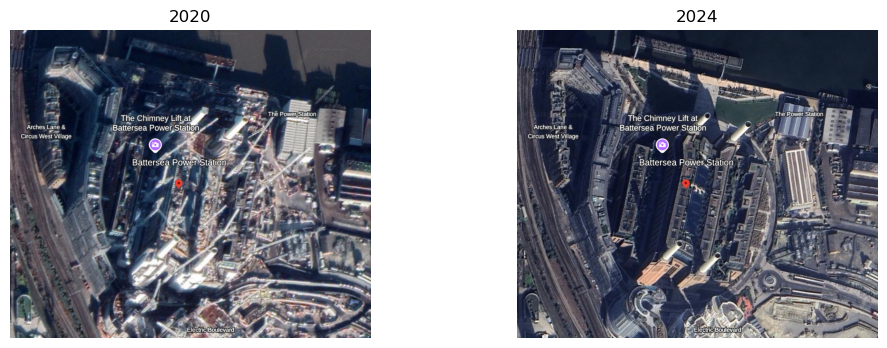
TipHome assignment
Who’s got more like Canary Wharf?
Footnotes
The figures below are screenshots from Google Earth, using its time travel tool (which is pretty cool).↩︎