# Geospatial Libraries
import pandas as pd
import geopandas as gpd
import numpy as np

# Plotting
import matplotlib.pyplot as pltPrecipitation - Exploring Rainfall Across the UK
Goal: Using the Imago precipitation product to explore rainfall across the UK, discovering the wettest and driest MSOAs and the regional precipitation characteristics.
Data:
NoteInstalling the data
The Imago precipitation data is hosted on the data catalogue. To download it:
- Sign up for a free account on the data catalogue and log in.
- Search for
precipitation MSOA(or browse the precipitation datasets). - Open the data link, Precipitation per MSOA in 2024, and download the
.gpkgfile. - Save the files into a
../data/folder in your project, keeping the original filenames (precipitation_indicators_MSOA_2024.gpkg).
For this notebook, you’ll need the 2024 MSOA file, and then repeat for the 2024 LAD file.
A question to motivate the data
A local authority believes that 2024 was an exceptionally wet year. Before investigating whether rainfall was unusual, we first need to understand how rainfall was distributed across the UK and whether wet conditions were concentrated in specific regions or spread more evenly across the country.
Installing Libraries
We install core geospatial libraries needed for this work.
Loading the Data
Using geopandas, we can read the gpkg. As it’s a gpkg it already has the geometric shape of the areas (in the geometry column) and will not need a separate boundary file.
precip_msoa = gpd.read_file("data/precipitation_indicators_MSOA_2024.gpkg")
precip_msoa.head()| dt_zn_c | dt_zn_n | rainfall_annual_mm | winter_rainfall | spring_rainfall | summer_rainfall | autumn_rainfall | annual_anomaly_abs | annual_anomaly_std | extreme_days_4sd | year | geometry | |
|---|---|---|---|---|---|---|---|---|---|---|---|---|
| 0 | E02000001 | City of London 001 | 696.647095 | 223.671677 | 189.220276 | 107.580292 | 218.248856 | 158.290131 | 2.148560 | 26.304880 | 2024 | MULTIPOLYGON (((532135.138 182198.131, 532158.... |
| 1 | E02000002 | Barking and Dagenham 001 | 695.338257 | 236.243835 | 192.781601 | 106.833694 | 205.600983 | 131.554367 | 1.715453 | 23.520077 | 2024 | MULTIPOLYGON (((548881.563 190845.265, 548881.... |
| 2 | E02000003 | Barking and Dagenham 002 | 667.498779 | 230.828064 | 185.345505 | 100.507462 | 195.728653 | 120.716499 | 1.595210 | 22.027685 | 2024 | MULTIPOLYGON (((549102.438 189324.625, 548954.... |
| 3 | E02000004 | Barking and Dagenham 003 | 611.439758 | 218.056824 | 171.161316 | 89.372581 | 175.921600 | 93.010658 | 1.238803 | 23.146259 | 2024 | MULTIPOLYGON (((551550.056 187364.705, 551478 ... |
| 4 | E02000005 | Barking and Dagenham 004 | 632.301819 | 224.054337 | 176.073090 | 93.059616 | 183.112747 | 102.117798 | 1.371893 | 22.568747 | 2024 | MULTIPOLYGON (((549099.634 187656.076, 549161.... |
This file contains multiple rainfall indicators. For this notebook we use the following two:
rainfall_annual_mm: Average yearly rainfall depth in mm. It measures the average depth of rain that fell across a specific local area (MSOA) during the year, rather than a total volume.geometry: spatial boundaries for each MSOA.
Understanding the Distribution of Rainfall
Before mapping the data locally, it is useful to look at the national summary statistics. These provide a high-level overview of the rainfall conditions observed across the whole of the UK during 2024.
(precip_msoa[["rainfall_annual_mm"]].agg(["mean", "std", "min", "max"]))| rainfall_annual_mm | |
|---|---|
| mean | 972.689669 |
| std | 274.112145 |
| min | 516.364502 |
| max | 3140.853516 |
Rainfall is rarely distributed evenly. Some areas receive substantially more rainfall than others, and understanding this variation helps provide context for local claims about exceptionally wet conditions.
Calculating the bins
To calculate bins for the histograms Freedman-Diaconis rule is used because it adapts bin width based on the variability of the data while limiting the influence of outliers. This is suitable for rainfall related variables, where distributions can be skewed due to regional differences and extreme events.
# Freedman-Diaconis Calculations
data = precip_msoa["rainfall_annual_mm"]
data_points = len(data)
q1 = data.quantile(0.25)
q3 = data.quantile(0.75)

# Calculate interquartile range
iqr = q3 - q1

bin_width = (2 * iqr) / (data_points ** (1 / 3))

ann_rainfall_bins = int(np.ceil((data.max() - data.min()) / bin_width))
ann_rainfall_bins = round(ann_rainfall_bins, 0)
print(f"Amount of rainfall bins: {ann_rainfall_bins}")
Amount of rainfall bins: 92fig, ax = plt.subplots(1, figsize=(7, 4))
ax.hist(
precip_msoa["rainfall_annual_mm"].dropna(),
bins=ann_rainfall_bins,
edgecolor="black",
color="darkslategrey",
)
ax.set_title("Annual Rainfall (mm)", fontweight="bold")
ax.set_ylabel("Count")
ax.grid(axis="y", linestyle="--", alpha=0.3)
ax.grid(axis="x", visible=False)
fig.suptitle("Distribution of rainfall exposure across MSOAs, 2024", fontweight="bold")
plt.tight_layout()
plt.show()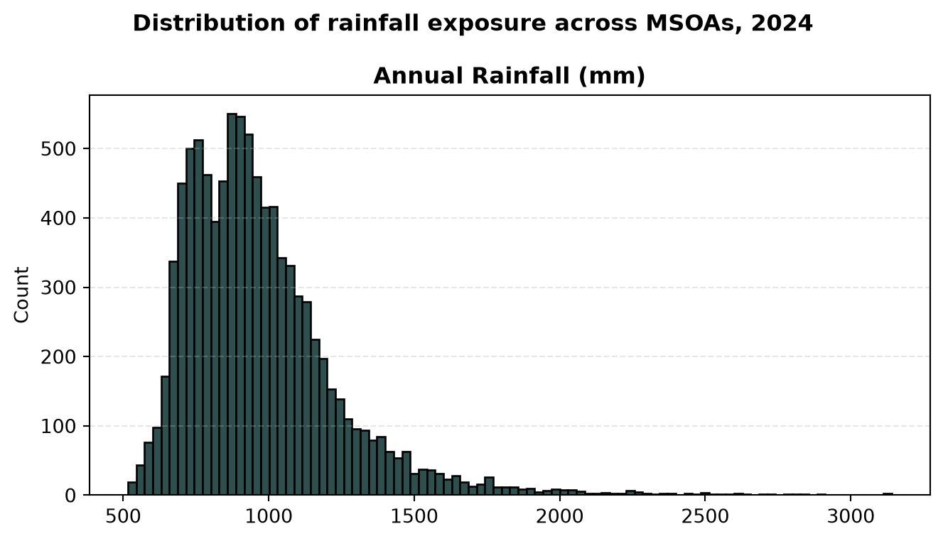
NoteInterpretation
The distribution is positively skewed, with most MSOAs clustered around moderate rainfall totals and a smaller number of particularly wet locations extending the upper tail of the distribution. This is highlighting how the majority of MSOAs experience a relatively low amount of rainfall however the rainfall countrywide varies with a tail of progressively higher means.
Finding the extreme MSOAs
One simple way to understand rainfall concentration is to rank areas by total annual rainfall.
wettest = precip_msoa.nlargest(10, "rainfall_annual_mm")[
    ["dt_zn_c", "dt_zn_n", "rainfall_annual_mm"]
]
driest = precip_msoa.nsmallest(10, "rainfall_annual_mm")[
    ["dt_zn_c", "dt_zn_n", "rainfall_annual_mm"]
]

print("Wettest MSOAs, 2024:")
print(wettest.to_string(index=False))

print("\nDriest MSOAs, 2024:")
print(driest.to_string(index=False))
Wettest MSOAs, 2024:
dt_zn_c dt_zn_n rainfall_annual_mm
E02003976 Allerdale 012 3140.853516
E02004015 South Lakeland 001 3128.609863
W02000258 Rhondda Cynon Taf 007 3121.053467
S02003309 Lochalsh 2909.670654
W02000261 Rhondda Cynon Taf 010 2838.054199
S02003281 Fort William South 2818.538086
W02000262 Rhondda Cynon Taf 011 2793.097412
S02003310 Skye South 2776.712891
W02000260 Rhondda Cynon Taf 009 2737.283691
S02003279 Lochaber West 2706.211182
Driest MSOAs, 2024:
dt_zn_c dt_zn_n rainfall_annual_mm
E02003291 Southend-on-Sea 013 516.364502
E02003311 Thurrock 016 517.631042
E02003304 Thurrock 009 517.999329
E02005010 Canterbury 001 519.244873
E02006926 Thurrock 020 523.255981
E02005011 Canterbury 002 523.720581
E02007005 Thurrock 022 527.915466
E02006859 Thurrock 019 530.438965
E02003312 Thurrock 017 530.513855
E02004560 Maldon 006 530.607605
NoteOutliers
A single year’s ranking is sensitive to one unusual season. An MSOA at the top of this list in 2024 or the bottom of this list is solely for this year, and it does not reveal if it is part of a bigger regional pattern, a specific seasonal spike or just an isolated high rainfall year.
Mapping rainfall by local area
Mapping rainfall reveals the spatial structure hidden within the rankings. Neighbouring MSOAs often experience similar conditions, producing regional rainfall patterns that are not obvious from tables alone.
fig, ax = plt.subplots(1, figsize=(8, 6))

precip_msoa.plot(
    column="rainfall_annual_mm",
    cmap="Blues",
    legend=True,
    ax=ax,
    linewidth=0,
    legend_kwds={"shrink": 0.5, "label": "mm"},
)
ax.set_title("Annual rainfall", fontweight="bold")
ax.set_axis_off()

fig.suptitle("Rainfall exposure across MSOAs, 2024", fontweight="bold")
plt.tight_layout()
plt.show()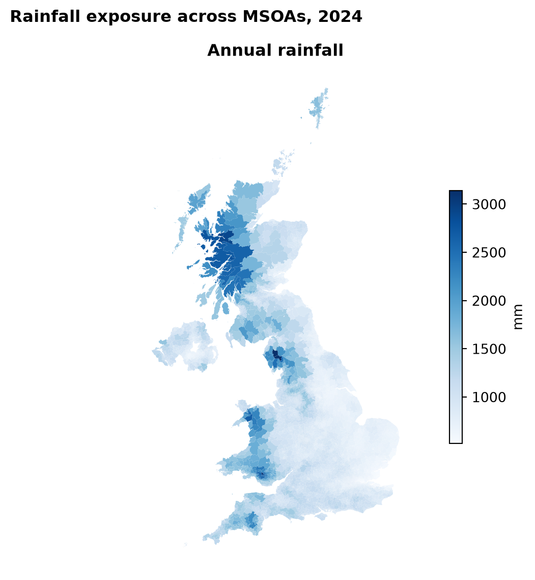
Patterns
Beyond serving as a useful sanity check, mapping the data reveals spatial patterns that highlight regional variations in rainfall. We can clearly see that certain parts of the country get lots of rainfall (Scotland, Lancashire, and Wales) while other parts such as the south of England do not. We can see a clear southeast-to-northwest gradient of increasing rainfall.
Regional differences
So far we’ve looked at MSOAs. Imago also publishes a LAD level version of the same precipitation product with rainfall computed directly at the local authority level, rather than something we would have to derive ourselves by averaging MSOAs up. Using this pre-aggregated product is much simpler than trying to average MSOA values ourselves.
Loading LAD Data
This data is loaded in the same way as the MSOA data, and since it is in GeoPackage (.gpkg) format, it already includes the boundaries. We print the first observations of the dataset to inspect its structure.
precip_lad = gpd.read_file("data/precipitation_indicators_LAD_2024.gpkg")
precip_lad.head()| LAD21CD | LAD21NM | rainfall_annual_mm | winter_rainfall | spring_rainfall | summer_rainfall | autumn_rainfall | annual_anomaly_abs | annual_anomaly_std | extreme_days_4sd | year | geometry | |
|---|---|---|---|---|---|---|---|---|---|---|---|---|
| 0 | E06000001 | Hartlepool | 686.761658 | 217.900101 | 194.122314 | 140.255630 | 175.145996 | 110.656914 | 1.173922 | 21.315712 | 2024 | MULTIPOLYGON (((447213.9 537036.104, 447206.00... |
| 1 | E06000002 | Middlesbrough | 741.491333 | 192.090210 | 209.281387 | 154.297791 | 201.528397 | 119.056717 | 1.304255 | 19.883654 | 2024 | MULTIPOLYGON (((448609.9 521982.6, 448586.35 5... |
| 2 | E06000003 | Redcar and Cleveland | 865.258606 | 225.683945 | 230.743408 | 182.541229 | 234.379837 | 159.905365 | 1.732852 | 20.556686 | 2024 | MULTIPOLYGON (((455932.335 527880.697, 455939.... |
| 3 | E06000004 | Stockton-on-Tees | 693.715271 | 203.911972 | 199.658813 | 135.914932 | 192.368607 | 104.323410 | 1.147774 | 20.970232 | 2024 | MULTIPOLYGON (((444157.002 527956.304, 444139.... |
| 4 | E06000005 | Darlington | 716.726807 | 240.145233 | 214.126801 | 129.527863 | 199.460587 | 90.094154 | 0.950165 | 20.299484 | 2024 | MULTIPOLYGON (((423496.602 524724.299, 423475.... |
To examine the extremes of the distribution, we look at the wettest and driest local authorities in 2024.
wettest_lad = precip_lad.nlargest(10, "rainfall_annual_mm")[
    ["LAD21CD", "LAD21NM", "rainfall_annual_mm"]
]

driest_lad = precip_lad.nsmallest(10, "rainfall_annual_mm")[
    ["LAD21CD", "LAD21NM", "rainfall_annual_mm"]
]

print("Wettest local authorities, 2024:")
print(wettest_lad.to_string(index=False))
print("Driest local authorities, 2024:")
print(driest_lad.to_string(index=False))
Wettest local authorities, 2024:
LAD21CD LAD21NM rainfall_annual_mm
W06000016 Rhondda Cynon Taf 2264.987793
E07000031 South Lakeland 2228.302002
W06000012 Neath Port Talbot 2155.255127
S12000035 Argyll and Bute 2122.896973
E07000029 Copeland 2113.462891
W06000002 Gwynedd 2104.406250
W06000013 Bridgend 2029.671753
S12000030 Stirling 2024.052734
W06000024 Merthyr Tydfil 1982.400146
S12000017 Highland 1925.752808
Driest local authorities, 2024:
LAD21CD LAD21NM rainfall_annual_mm
E07000075 Rochford 565.752625
E06000033 Southend-on-Sea 568.152588
E07000074 Maldon 569.419800
E07000114 Thanet 579.956970
E06000034 Thurrock 584.442139
E07000069 Castle Point 584.549500
E07000076 Tendring 598.346802
E09000002 Barking and Dagenham 619.939941
E07000071 Colchester 624.941345
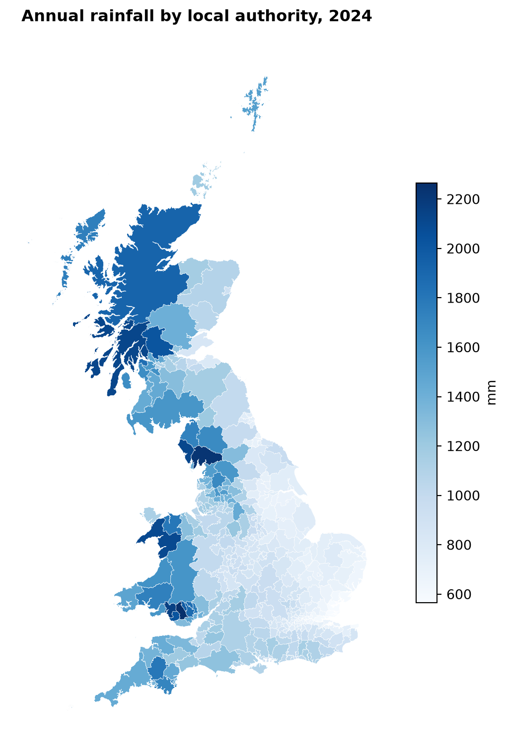
E09000016 Havering 633.256348We can create a horizontal bar chart comparing the 15 wettest and 15 driest local authorities to highlight the absolute differences between the extremes. We then generate a choropleth map of the UK to show how this annual rainfall is distributed geographically across all local authorities.
fig, ax = plt.subplots(figsize=(7, 10))

lad_sorted = precip_lad.sort_values("rainfall_annual_mm", ascending=False)
top_bottom = pd.concat([lad_sorted.head(15), lad_sorted.tail(15)])

ax.barh(top_bottom["LAD21NM"], top_bottom["rainfall_annual_mm"], color="darkslategrey")
ax.set_xlabel("Annual rainfall (mm)")
ax.set_title("Local authorities: wettest and driest 15, 2024", fontweight="bold")
ax.invert_yaxis()
plt.tight_layout()
plt.show()

fig, ax = plt.subplots(figsize=(7, 8))

precip_lad.plot(
    column="rainfall_annual_mm",
    cmap="Blues",
    legend=True,
    ax=ax,
    linewidth=0.2,
    edgecolor="white",
    legend_kwds={"shrink": 0.6, "label": "mm"},
)
ax.set_title("Annual rainfall by local authority, 2024", fontweight="bold")
ax.set_axis_off()

plt.tight_layout()
plt.show()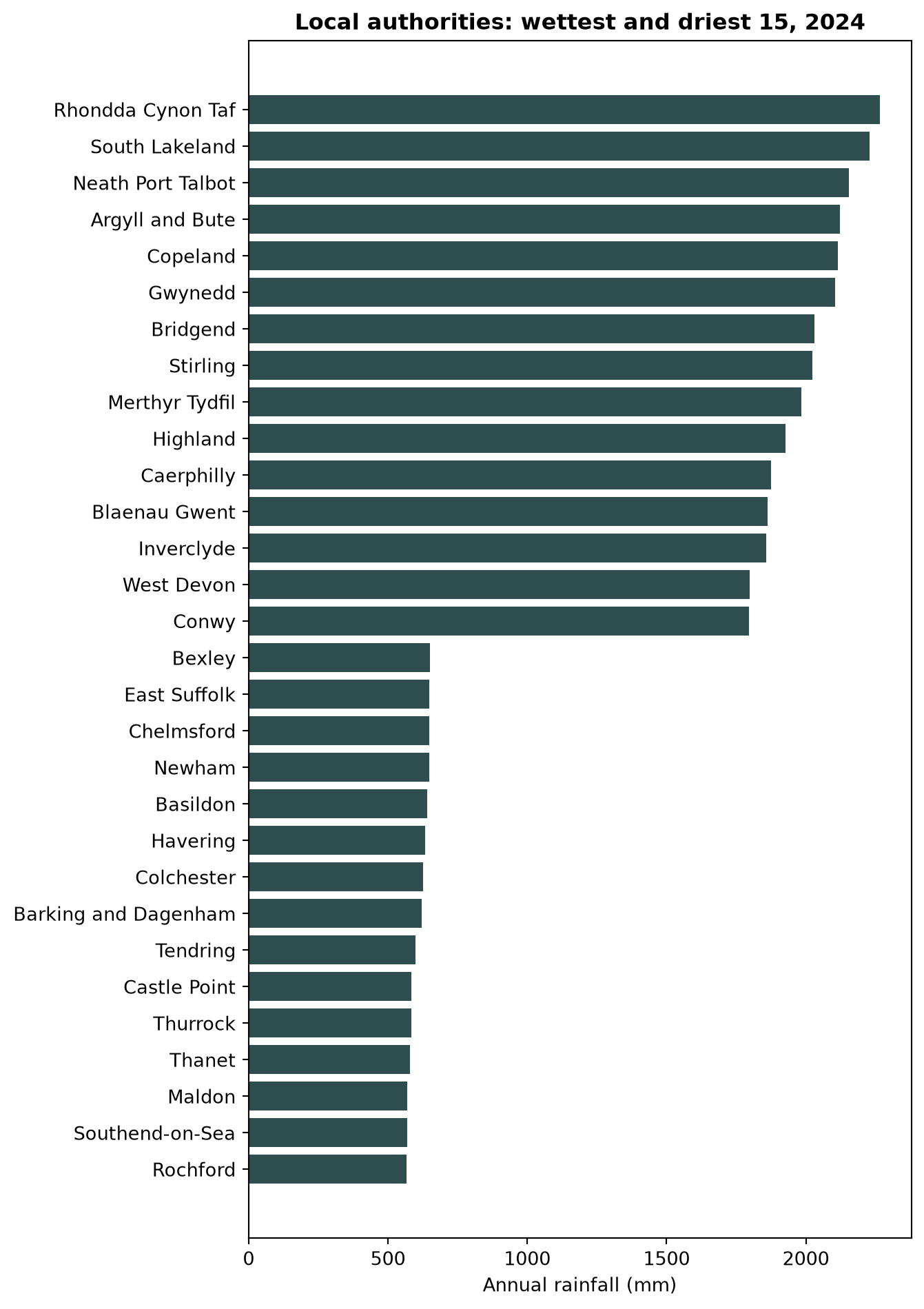
Comparing the two scales
Next, we examine whether the trends observed at the LAD level align with the finer-grained MSOA patterns. If a LAD ranks among the wettest, do its individual MSOAs from earlier in the notebook also sit toward the top of the MSOA ranking? Alignment between these levels confirms that regional trends are representative of the area, rather than being driven by isolated outliers that distort the local authority average. Divergence between the two scales is also valuable; a local authority with near-average overall rainfall might still contain an individual MSOA with extreme exposure, which would be obscured by the aggregate LAD average alone
Mapping the gap between scales
We can visualise this comparison by mapping the deviation of each MSOA’s rainfall from its local authority’s average. A value close to zero means the MSOA is typical of its local authority district, while large positive or negative values highlight localised areas with unusually high or low rainfall compared to the regional average.
# Spatial overlay in order to compare
msoa_lad_overlap = gpd.overlay(
    precip_msoa[["dt_zn_c", "geometry"]],
    precip_lad[["LAD21CD", "LAD21NM", "rainfall_annual_mm", "geometry"]].rename(
        columns={"rainfall_annual_mm": "lad_rainfall_annual_mm"}
    ),
    how="intersection",
    keep_geom_type=False,
)

# Keep the LAD each MSOA overlaps with most, by area
msoa_lad_overlap["overlap_area"] = msoa_lad_overlap.geometry.area
best_match = msoa_lad_overlap.sort_values(
    "overlap_area", ascending=False
).drop_duplicates(subset="dt_zn_c", keep="first")[
    ["dt_zn_c", "LAD21CD", "LAD21NM", "lad_rainfall_annual_mm"]
]

msoa_with_lad = precip_msoa.merge(best_match, on="dt_zn_c", how="left")

n_unmatched = msoa_with_lad["LAD21CD"].isna().sum()
print(
    f"{n_unmatched} MSOAs have no matching LAD (The North of Ireland is not covered by the LAD precipitation product)"
)

msoa_with_lad = msoa_with_lad.dropna(subset=["LAD21CD"])

msoa_with_lad["rainfall_diff"] = (
    msoa_with_lad["rainfall_annual_mm"] - msoa_with_lad["lad_rainfall_annual_mm"]
)

# Clip the colour scale to the 1st/99th percentile rather than true min/max
# A small number of genuine outliers (like large, internally varied Highland LADs) would compress the entire typical range into a narrow band near white.
# Outliers beyond this range are still shown, just fully saturated.
p01 = msoa_with_lad["rainfall_diff"].quantile(0.01)
p99 = msoa_with_lad["rainfall_diff"].quantile(0.99)
diff_limit = max(abs(p01), abs(p99))

fig, ax = plt.subplots(figsize=(9, 9))
fig.patch.set_facecolor("#dfdddd")
ax.set_facecolor("#dfdddd")

msoa_with_lad.plot(
    column="rainfall_diff",
    cmap="RdBu",
    legend=True,
    ax=ax,
    linewidth=0,
    vmin=-diff_limit,
    vmax=diff_limit,
    legend_kwds={
        "shrink": 0.6,
        "label": "mm (MSOA - parent LAD, clipped at 1st/99th pct)",
    },
)
ax.set_title(
    "MSOA rainfall relative to its own local authority, 2024", fontweight="bold"
)
ax.set_axis_off()
plt.tight_layout()
plt.show()

extremes = msoa_with_lad.nlargest(3, "rainfall_diff")[["dt_zn_n", "rainfall_diff"]]
print(extremes.to_string(index=False))

extremes_low = msoa_with_lad.nsmallest(3, "rainfall_diff")[["dt_zn_n", "rainfall_diff"]]
print(extremes_low.to_string(index=False))
850 MSOAs have no matching LAD (The North of Ireland is not covered by the LAD precipitation product)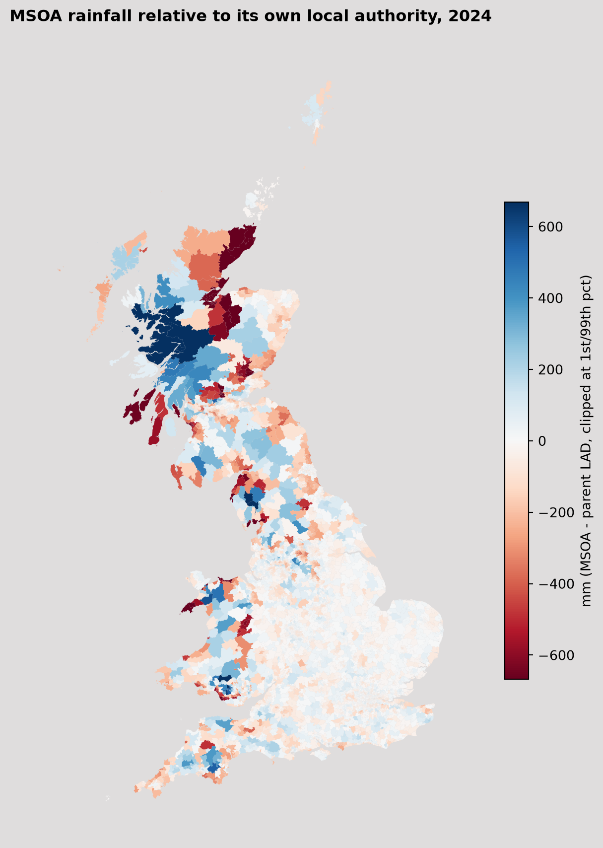
           dt_zn_n  rainfall_diff
     Allerdale 012    1412.004883
          Lochalsh     983.917847
South Lakeland 001     900.307861
           dt_zn_n  rainfall_diff
          Seaboard   -1134.862122
Inverness Merkinch   -1107.408691
Inverness Muirtown   -1092.341003
Note
Most MSOAs sit close to their LAD’s average, appearing pale across much of England. Scotland and Wales are the exception with Lochalsh sitting 984 mm above its LAD average while Inverness sits 1107 mm below. These larger, more topographically varied local authorities can contain substantial rainfall differences within a single administrative boundary. England’s generally smaller LADs show less internal variation.
This highlights an important point when interpreting regional rainfall statistics. A local authority average can provide a useful summary of overall conditions, but it may also hide variation between individual communities. Looking at both MSOA and LAD scales helps reveal whether rainfall patterns are widespread across an authority or concentrated in particular areas.
What have we learnt?
This first case study explored how rainfall was distributed across the UK during 2024.
Understanding where rainfall was concentrated is the first step in investigating claims about exceptionally wet conditions. However, annual rainfall totals alone do not explain why an area was wet.
Two places can record similar annual rainfall totals while experiencing very different seasonal patterns. One may receive rainfall steadily throughout the year, while another may be heavily influenced by a particularly wet season.
We found that:
- Rainfall is not evenly distributed across the country.
- Clear regional patterns emerge when rainfall is mapped.
- There are multiple ways to identify rainfall extremes, such as sorting rankings or visualising patterns on a map.
- Local authority averages capture broad regional trends, but can sometimes mask variation between individual MSOAs.
In the next case study, we break annual rainfall into spring, summer, autumn, and winter totals to investigate what drove rainfall patterns across the UK during 2024.