# Geospatial Libraries
import pandas as pd
import geopandas as gpd

# Plotting
import matplotlib.pyplot as pltPrecipitation - Flood Exposure and Flood Risk
Data:
Goal: Using the Imago precipitation product alongside the Imago flooding product and Census population estimates, identify which communities in Yorkshire and Humber combine unusually wet conditions with high flood exposure and large resident populations.
NoteInstalling the data
Unlike the previous case studies, this notebook combines two Imago products with census population estimates and county boundaries to create the study region. For the region boundaries install the gpkg. The precipitation and flooding products can both be downloaded directly from Imago. The only external dataset required is the Census population estimates.
Census Data
Population estimates are taken from the 2021 Census at MSOA level. Download the dataset from the Office for National Statistics using the following options:
Geography: - England and Wales - 2021 Middle Layer Super Output Areas (MSOAs)
Residence type: - Total: All usual residents
Output: - Value
Format: - Excel (.xlsx)
Place the downloaded spreadsheet inside the data/ directory.
The Reason for the Data
In the previous case studies we explored where rainfall occurred, how it varied through the seasons, and which places experienced unusually wet conditions relative to the historical climate. While interesting from a climatological perspective, rainfall alone tells us little about its potential impact on society.
Flooding provides one example where environmental conditions become socially significant. Heavy rainfall is most likely to create disruption where communities are also located within areas that are susceptible to flooding. In this notebook we combine three different datasets:
- rainfall anomalies from the Imago precipitation product.
- flood exposure from the Imago flooding product.
- Census population estimates.
Together these allow us to identify communities that experienced unusually wet conditions, have meaningful flood exposure, and contain substantial resident populations.
Installing Libraries
Defining the Study Area
Unlike the previous case studies, this notebook combines several geospatial datasets. The flood product contains polygons covering the whole of the UK, while the Census provides population estimates for every MSOA.
Although the Imago datasets are much smaller than the original national datasets from which they were derived, they still cover every MSOA in England or the UK. Restricting the analysis to Yorkshire and the Humber reduces processing time and allows us to focus on a region containing large urban centres, major river systems and varied rainfall patterns.
regions = gpd.read_file("data/Regions_Dec_2020_EN_BGC_2022_-724820876220737106.gpkg")

regions.head()| RGN20CD | RGN20NM | BNG_E | BNG_N | LONG | LAT | GlobalID | geometry | |
|---|---|---|---|---|---|---|---|---|
| 0 | E12000001 | North East | 417314 | 600356 | -1.72888 | 55.297009 | {47370864-3D24-4F97-9CB5-8CBEE2F1985F} | MULTIPOLYGON (((402039.597 506235.701, 402144.... |
| 1 | E12000002 | North West | 350014 | 506279 | -2.77239 | 54.449440 | {8F0EB150-C5EA-4B13-BB4D-348170201C80} | MULTIPOLYGON (((312902.609 555602.337, 312908.... |
| 2 | E12000003 | Yorkshire and The Humber | 446902 | 448736 | -1.28714 | 53.932640 | {CA39CDD0-E4D2-4AF3-932E-6B95FC6F8C7B} | MULTIPOLYGON (((450524.201 378564.296, 450605.... |
| 3 | E12000004 | East Midlands | 477659 | 322635 | -0.84969 | 52.795719 | {484FF822-37BE-4798-8EB7-B88C484E8DF1} | MULTIPOLYGON (((455182.298 231283.095, 455301.... |
| 4 | E12000005 | West Midlands | 386294 | 295477 | -2.20358 | 52.556969 | {00750B56-C8A0-4663-B3D9-373A02DA1FA4} | MULTIPOLYGON (((403387.797 368314.9, 402988.2 ... |
study_area = regions[regions["RGN20NM"] == "Yorkshire and The Humber"]

fig, ax = plt.subplots(figsize=(6, 8))

study_area.plot(
    ax=ax,
    color="lightgrey",
    edgecolor="black",
)

ax.set_title("Study Area")
ax.axis("off")

plt.show()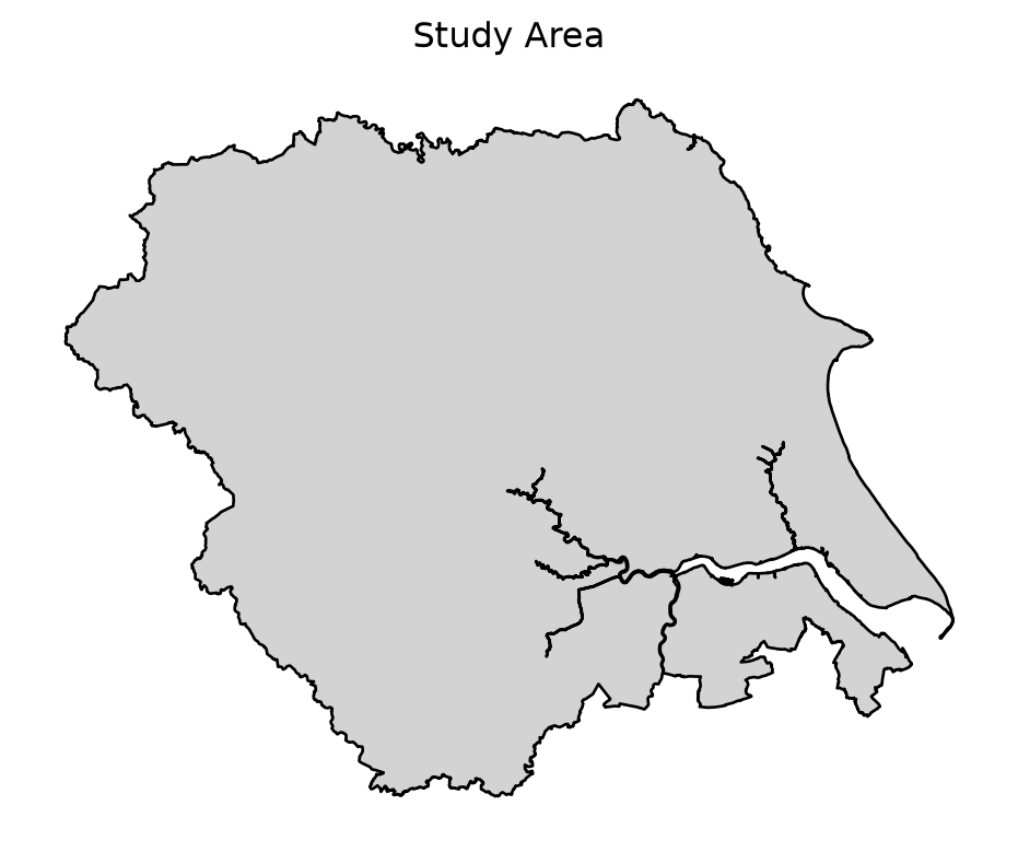
As we can see, the Yorkshire and The Humber region is cleanly marked out and has no visible problems. We now need to apply this to our data.
Loading the data
The precipitation product and national flood zone dataset contain information for the whole of the UK and England respectively. For many analyses this is appropriate, however loading the entire datasets consumes unnecessary memory and processing time when we are only interested in one region.
GeoPandas allows us to read only the features intersecting our study area by supplying a spatial mask during loading. This is much faster and is a common approach when working with large spatial datasets.
# Imago precipitation product
precip = gpd.read_file(
    "data/precipitation_indicators_MSOA_2021.gpkg",
    mask=study_area,
)

# Environment Agency Flood Zones
flood = gpd.read_file(
    "data/flood_indicators_MSOA_2021.gpkg",
    mask=study_area,
)

# Census population
population = pd.read_excel(
    "data/nomis_2026_07_06_155344.xlsx",
    skiprows=8,
    names=["area", "population"],
)
/opt/hostedtoolcache/Python/3.12.13/x64/lib/python3.12/site-packages/openpyxl/styles/stylesheet.py:237: UserWarning: Workbook contains no default style, apply openpyxl's default
warn("Workbook contains no default style, apply openpyxl's default")
Note
As NOMIS excel spreadsheets can be rather annoying in metadata and information, we need to clean it up.
population = population[population["area"].str.startswith("msoa2021:")].copy()

population["MSOA21CD"] = population["area"].str.extract(r"(E\d{8}|W\d{8})")

population["MSOA21NM"] = (
    population["area"]
    .str.replace(r"msoa2021:E\d{8}\s:\s", "", regex=True)
    .str.replace(r"msoa2021:W\d{8}\s:\s", "", regex=True)
)

population = population[["MSOA21CD", "MSOA21NM", "population"]]

population.head()| MSOA21CD | MSOA21NM | population | |
|---|---|---|---|
| 0 | E02002483 | Hartlepool 001 | 10239.0 |
| 1 | E02002484 | Hartlepool 002 | 10278.0 |
| 2 | E02002485 | Hartlepool 003 | 8001.0 |
| 3 | E02002489 | Hartlepool 007 | 7125.0 |
| 4 | E02002490 | Hartlepool 008 | 5805.0 |
Joining Population to the Precipitation Data
The precipitation indicators describe weather conditions for each MSOA, while the census provides the resident population for the same geography. We can combine these datasets using the MSOA code so that each area has both rainfall information and its resident population.
We can also clean the dataset to solely have the required data we are using.
precip = precip.rename(
    columns={
        "dt_zn_c": "MSOA21CD",
        "dt_zn_n": "MSOA21NM",
    }
)
precip = precip[
    [
        "MSOA21CD",
        "MSOA21NM",
        "annual_anomaly_std",
        "rainfall_annual_mm",
        "geometry",
    ]
]

flood = flood.rename(columns={"dt_zn_c": "MSOA21CD"})
flood = flood.drop(columns="geometry")

msoa = precip.merge(
    flood[
        [
            "MSOA21CD",
            "dummy_flooded",
            "flooded_area_km2_FZ2and3",
            "flooded_area_km2_FZ3",
            "ratio_flooded_total",
        ]
    ],
    on="MSOA21CD",
    how="left",
).merge(
    population[["MSOA21CD", "population"]],
    on="MSOA21CD",
    how="left",
)

msoa.head()| MSOA21CD | MSOA21NM | annual_anomaly_std | rainfall_annual_mm | geometry | dummy_flooded | flooded_area_km2_FZ2and3 | flooded_area_km2_FZ3 | ratio_flooded_total | population | |
|---|---|---|---|---|---|---|---|---|---|---|
| 0 | E02002658 | Kingston upon Hull 007 | 0.906769 | 657.062805 | MULTIPOLYGON (((512563.75 433676.719, 512475.1... | 1 | 0.900124 | 0.842844 | 0.570343 | 6547.0 |
| 1 | E02002673 | Kingston upon Hull 022 | 0.776747 | 658.475098 | MULTIPOLYGON (((511639 431206, 511921.999 4308... | 1 | 0.893939 | 0.893939 | 1.000000 | 7521.0 |
| 2 | E02002671 | Kingston upon Hull 020 | 0.789127 | 649.677673 | MULTIPOLYGON (((515978.702 428310.405, 515902.... | 1 | 6.713943 | 5.769255 | 0.900568 | 8977.0 |
| 3 | E02002662 | Kingston upon Hull 011 | 0.819893 | 653.184692 | MULTIPOLYGON (((513051 433055, 513011 433007, ... | 1 | 1.530689 | 1.472845 | 0.779522 | 7386.0 |
| 4 | E02002668 | Kingston upon Hull 017 | 0.770927 | 648.104309 | MULTIPOLYGON (((514603.438 431594.375, 514621.... | 1 | 1.840633 | 1.840633 | 1.000000 | 8400.0 |
Understanding the Flooding Product
Unlike the using the flooding data of the environmental agency, the Imago flooding product already summarises flood exposure for every MSOA.
For each area it provides:
- whether flooding is present.
- flooded area.
- the proportion of the MSOA lying within Flood Zones 2 and 3.
The main variables used in this notebook are:
dummy_flooded: Indicates whether any part of the MSOA intersects Flood Zones 2 or 3. A value of 1 means the MSOA contains some flood prone land.flooded_area_km2_FZ2and3: The total area (km²) within the MSOA that lies inside Flood Zones 2 or 3.ratio_flooded_total: The proportion of the MSOA’s total land area that lies within Flood Zones 2 or 3. Values range from 0 to 1, where 0.25 means 25% of the MSOA is within a flood zone.
msoa[
    [
        "MSOA21NM",
        "ratio_flooded_total",
        "flooded_area_km2_FZ2and3",
        "dummy_flooded",
    ]
].head()| MSOA21NM | ratio_flooded_total | flooded_area_km2_FZ2and3 | dummy_flooded | |
|---|---|---|---|---|
| 0 | Kingston upon Hull 007 | 0.570343 | 0.900124 | 1 |
| 1 | Kingston upon Hull 022 | 1.000000 | 0.893939 | 1 |
| 2 | Kingston upon Hull 020 | 0.900568 | 6.713943 | 1 |
| 3 | Kingston upon Hull 011 | 0.779522 | 1.530689 | 1 |
| 4 | Kingston upon Hull 017 | 1.000000 | 1.840633 | 1 |
Summary statistics
msoa["ratio_flooded_total"].describe()count 746.000000
mean 0.159463
std 0.254171
min 0.000000
25% 0.012438
50% 0.051713
75% 0.163463
max 1.000000
Name: ratio_flooded_total, dtype: float64
Note
These statistics show how flood exposure varies considerably across the region. Most MSOAs have little or no flood prone land, while some contain substantial proportions within Flood Zones 2 and 3, with some MSOAs being entirely flood prone.
Mapping Rainfall Anomalies
fig, ax = plt.subplots(figsize=(10, 10))

msoa.plot(
    column="annual_anomaly_std",
    cmap="Blues",
    legend=True,
    ax=ax,
)

ax.set_title("Rainfall Anomaly Relative to the Historical Average (2021)")
ax.axis("off")

plt.show()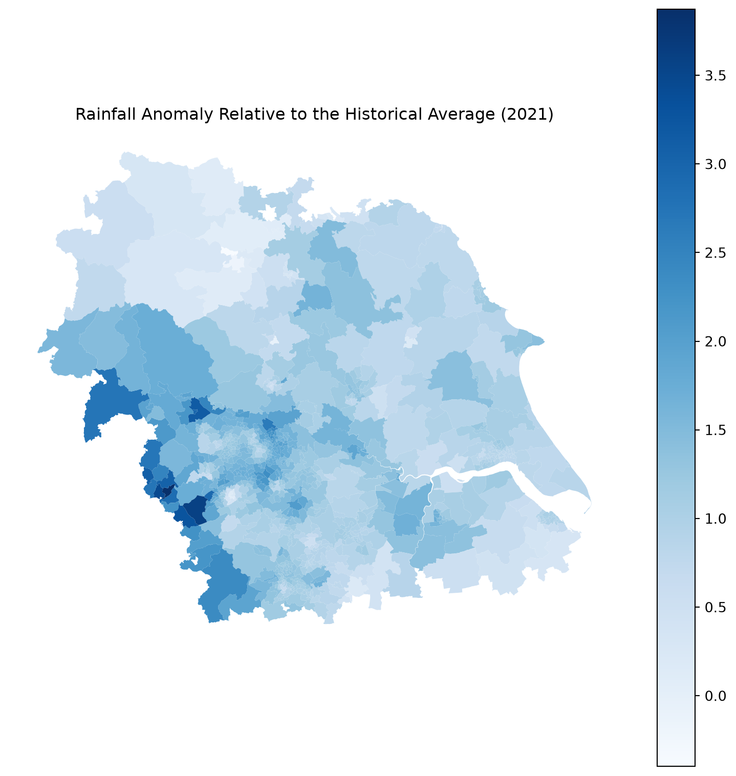
:::
Mapping Flood Exposure
fig, ax = plt.subplots(figsize=(10, 10))

msoa.plot(
    column="ratio_flooded_total",
    cmap="OrRd",
    legend=True,
    ax=ax,
)
study_area.boundary.plot(
    ax=ax,
    color="black",
    linewidth=0.5,
)

ax.set_title("Flood Exposure")
ax.axis("off")

plt.show()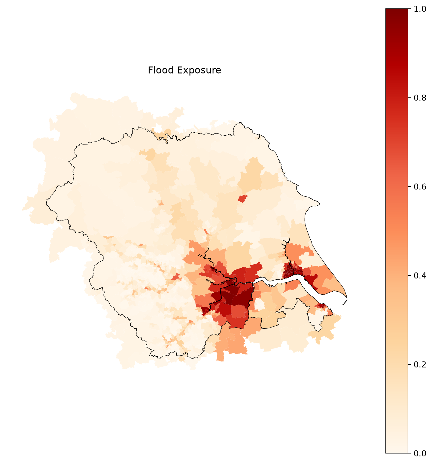
As we can see, flood exposure varies continuously with a concentration around the Humber. Darker areas indicate MSOAs where a larger proportion of land lies within Flood Zones 2 and 3.
Defining Potential Flood Exposure
Rather than considering every MSOA with even a very small amount of flood prone land, we define meaningful flood exposure as MSOAs where at least 10% of the area lies within Flood Zones 2 and 3.
threshold = 0.10

msoa["in_flood_zone"] = msoa["ratio_flooded_total"] >= threshold

msoa["high_anomaly"] = msoa["annual_anomaly_std"] > 1

msoa["category"] = "Neither"

msoa.loc[
    msoa["high_anomaly"],
    "category",
] = "High rainfall anomaly"

msoa.loc[
    msoa["in_flood_zone"],
    "category",
] = "Flood zone"

msoa.loc[
    msoa["high_anomaly"] & msoa["in_flood_zone"],
    "category",
] = "Both"

print(f"No flood exposure: {len(msoa[msoa['category'] == 'Neither'])}")
print(
    f"High rainfall anomaly: {len(msoa[msoa['category'] == 'High rainfall anomaly'])}"
)
print(f"Flood zone: {len(msoa[msoa['category'] == 'Flood zone'])}")
print(f"Both high anomaly and Floodzone: {len(msoa[msoa['category'] == 'Both'])}")
No flood exposure: 124
High rainfall anomaly: 357
Flood zone: 111
Both high anomaly and Floodzone: 154Mapping Potential Flood Exposure
colours = {
    "Neither": "grey",
    "High rainfall anomaly": "orange",
    "Flood zone": "blue",
    "Both": "red",
}

fig, ax = plt.subplots(figsize=(8, 8))

for category, colour in colours.items():

    msoa[msoa["category"] == category].plot(
        ax=ax,
        color=colour,
        edgecolor="white",
        linewidth=0.15,
        label=category,
    )

study_area.boundary.plot(
    ax=ax,
    color="black",
    linewidth=0.5,
)

ax.set_title("Potential Flood Exposure")

ax.axis("off")
ax.legend()

plt.show()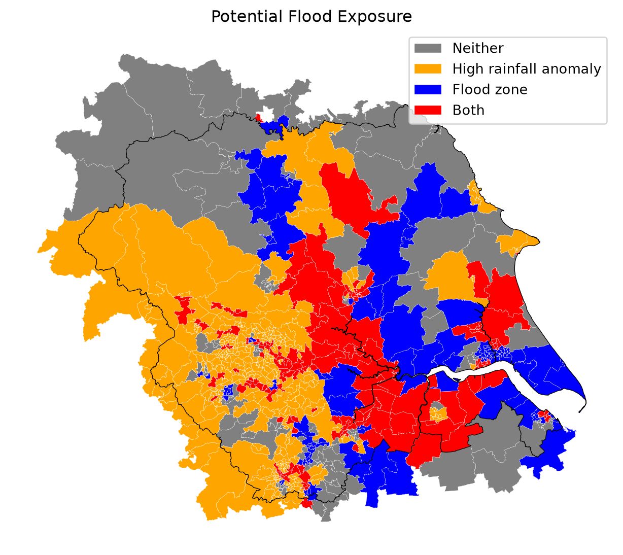
NoteInterpreting the Results
The combined map highlights four distinct groups of communities. Many MSOAs experienced unusually wet conditions during 2021 without substantial flood exposure especially in the west of the region, while parts of the region near rivers and the Humber are typical flood zones but did not receive anomalous rainfall.
Of greatest interest are the MSOAs classified as Both, where unusually wet conditions coincided with meaningful flood exposure. These areas may warrant additional investigation when considering flood resilience or future planning. While they are across most of the region, they are most concentrated around the Humber and its tributaries.
Population at Potential Flood Exposure
population_summary = msoa.groupby("category").agg(
    MSOAs=("MSOA21CD", "count"),
    Population=("population", "sum"),
)

population_summary| MSOAs | Population | |
|---|---|---|
| category | ||
| Both | 154 | 1272366.0 |
| Flood zone | 111 | 868294.0 |
| High rainfall anomaly | 357 | 2746818.0 |
| Neither | 124 | 1020970.0 |
We can see here that the total population of the region is ~5,9 million people, with 36% of the region being in a flood zone. Of that group, 60% experienced anomalous rainfall during 2021. While this is useful to know, it will be more insightful to see which MSOAs specifically were the highest population to make decisions.
Largest Potentially Exposed Communities
top = msoa[msoa["category"] == "Both"][
    [
        "MSOA21NM",
        "population",
        "annual_anomaly_std",
        "ratio_flooded_total",
    ]
].sort_values(
    "population",
    ascending=False,
)

top.head(20)| MSOA21NM | population | annual_anomaly_std | ratio_flooded_total | |
|---|---|---|---|---|
| 719 | Selby 005 | 13298.0 | 1.745343 | 0.931103 |
| 300 | Bradford 002 | 13119.0 | 1.330778 | 0.157497 |
| 111 | Leeds 055 | 12480.0 | 1.640491 | 0.121046 |
| 522 | Sheffield 022 | 12364.0 | 1.359429 | 0.371260 |
| 551 | Sheffield 075 | 12075.0 | 1.321252 | 0.166810 |
| 55 | North Lincolnshire 001 | 11921.0 | 1.062889 | 0.192663 |
| 288 | Bradford 008 | 11883.0 | 1.074736 | 0.173724 |
| 734 | Rotherham 027 | 11791.0 | 1.459730 | 0.256543 |
| 695 | Doncaster 022 | 11789.0 | 1.041220 | 0.305732 |
| 328 | York 019 | 11774.0 | 1.364767 | 0.153275 |
| 713 | Doncaster 003 | 11386.0 | 1.301867 | 0.793837 |
| 585 | Selby 004 | 11363.0 | 1.315923 | 0.190879 |
| 324 | York 013 | 11347.0 | 1.310723 | 0.259330 |
| 80 | Kirklees 024 | 11136.0 | 1.622244 | 0.352443 |
| 706 | Doncaster 009 | 10862.0 | 1.012055 | 0.296717 |
| 163 | Kingston upon Hull 031 | 10739.0 | 1.073758 | 0.984327 |
| 549 | Sheffield 073 | 10601.0 | 1.240555 | 0.246313 |
| 617 | Calderdale 025 | 10303.0 | 1.572555 | 0.109680 |
| 317 | York 012 | 10291.0 | 1.306614 | 0.108893 |
| 702 | Doncaster 015 | 10211.0 | 1.002988 | 0.434816 |
The twenty largest communities contain over two hundred thousand residents, illustrating that potential exposure is not distributed evenly across Yorkshire and the Humber. However, a list of communities alone does not tell us whether the majority of exposed residents live within the most flood prone MSOAs, or whether they are spread across many moderately exposed areas.
To investigate this, we now examine how the exposed population is distributed across different levels of flood exposure.
Population Distribution Across Flood Exposure Levels
Rather than considering flood exposure as simply present or absent, we divide MSOAs into groups according to the proportion of land that lies within Flood Zones 2 and 3.
bins = [0.10, 0.25, 0.50, float("inf")]

labels = [
    "10-25%",
    "25-50%",
    ">50%",
]

exposed = msoa[msoa["category"] == "Both"].copy()

exposed["Exposure Band"] = pd.cut(
    exposed["ratio_flooded_total"],
    bins=bins,
    labels=labels,
    include_lowest=True,
)

summary = exposed.groupby("Exposure Band").agg(
    MSOAs=("MSOA21CD", "count"),
    Population=("population", "sum"),
)

summary| MSOAs | Population | |
|---|---|---|
| Exposure Band | ||
| 10-25% | 79 | 656665.0 |
| 25-50% | 36 | 304520.0 |
| >50% | 39 | 311181.0 |
summary["Population"].plot(
    kind="bar",
    figsize=(7, 4),
    color="darkslategrey",
)

plt.title("Population Living in High Rainfall MSOAs by Flood Exposure")
plt.ylabel("Population")

plt.tight_layout()
plt.show()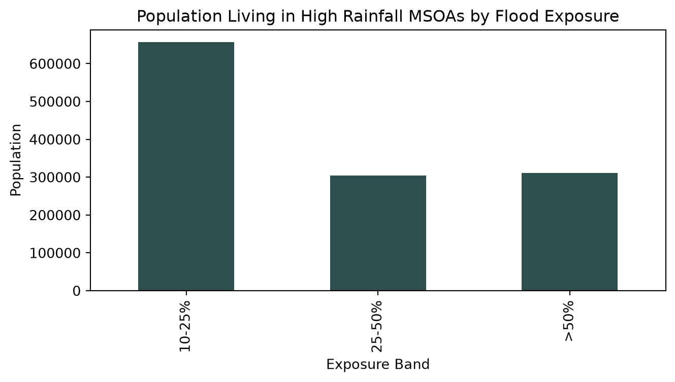
Note
The results indicate that the largest share of the exposed population is located within moderately flood-prone MSOAs (10–25% of the area at risk), rather than in those where over half of the land is flood prone. Consequently, flood resilience planning should not focus solely on the highest exposure areas, as substantial populations also reside within communities experiencing more moderate levels of flood exposure. Despite this you can see that half of the total population are living in 25%+ exposure MSOAs.
Identifying Priority Communities
Population alone does not fully describe potential flood exposure. A densely populated MSOA with only a small proportion of land at risk may require a different planning response from a similarly populated MSOA where most of the area lies within flood zones.
One simple way to identify communities that combine both characteristics is to calculate a potential exposure index by multiplying the resident population by the proportion of the MSOA that is classified as flood prone. While this is not a formal measure of flood risk, it provides a straightforward way of highlighting communities where large numbers of people coincide with extensive flood prone land.
msoa["potential_exposure"] = msoa["population"] * msoa["ratio_flooded_total"]

fig, ax = plt.subplots(figsize=(14, 14))

msoa[msoa["category"] == "Both"].plot(
    column="potential_exposure",
    cmap="OrRd",
    legend=True,
    edgecolor="white",
    linewidth=0.2,
    ax=ax,
)

study_area.boundary.plot(
    ax=ax,
    color="black",
    linewidth=0.5,
)

ax.set_title(
    "Potential Population Exposure",
    fontweight="bold",
)

ax.axis("off")

plt.tight_layout()
plt.show()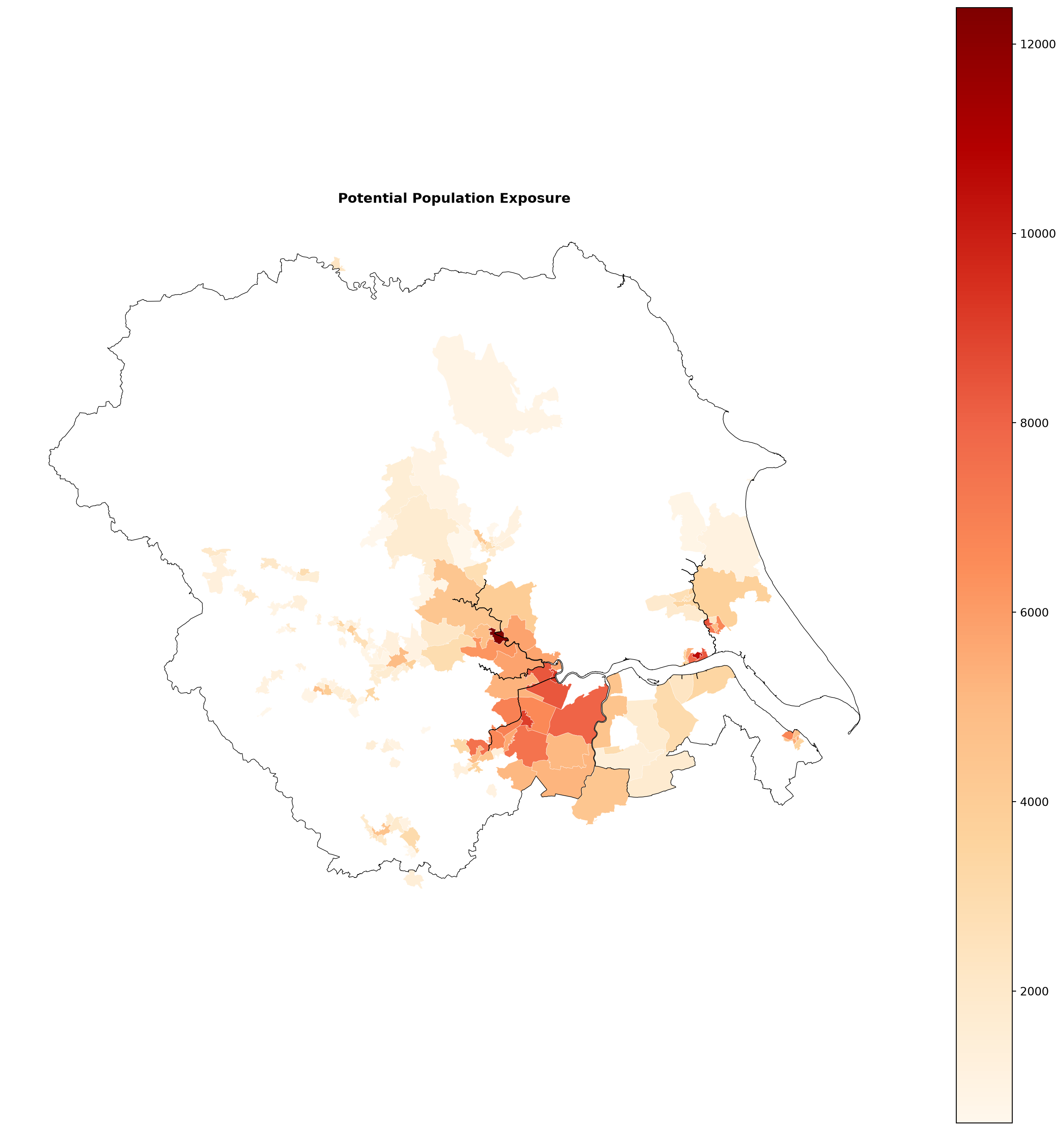
Note
The map identifies several clusters of communities with comparatively high potential population exposure, particularly across the central and southern parts of Yorkshire and the Humber.
These areas combine three characteristics:
- above average rainfall during 2021
- substantial proportions of land within Environment Agency flood zones
- relatively large resident populations
By contrast, many MSOAs with high rainfall contain relatively small populations or only limited flood prone land, reducing their overall potential societal exposure.The highest priority communities are not necessarily those receiving the most rainfall or those containing the largest flood extents, but those where environmental exposure and population coincide.
What have we learnt?
In this notebook we have:
- defined a regional study area before loading national datasets
- combined the Imago precipitation and flooding products with Census 2021 population estimates
- explored how rainfall anomalies varied across Yorkshire and the Humber
- identified communities that experienced both unusually wet conditions and meaningful flood exposure
- quantified how many MSOAs and residents fall within these communities
- identified the largest potentially exposed communities using simple population summaries
- demonstrated how environmental and demographic datasets can be combined to support spatial analysis