# Geospatial Datascience libraries
import geopandas as gpd
import numpy as np

# Plotting
from matplotlib.colors import TwoSlopeNorm
import matplotlib.pyplot as pltSun Probability Framework - Comparing 2024 and 2025
Data:
Goal: Compare the 2024 and 2025 Sun Probability Framework (SPF) products to identify how cloud cover conditions changed across the UK.
NoteDownload the data
Download both SPF datasets from the Imago Data Service.
Place both GeoPackages inside the data/ directory.
The datasets provide annual estimates of annual cloud probability for every small area across the United Kingdom.1 Therefore, this notebook focuses on the cloud_probability variable, which represents the annual average SPF value for these geographies.
What is Sun Probability Framework?
The Sun Probability Framework (SPF) summarises the probability of cloud cover obscuring the ground. Higher SPF values indicate cloudier conditions and therefore a lower likelihood of direct sunlight reaching the surface, while lower values indicate clearer conditions.
The Reason for the Data
Exposure to sunshine, and therefore cloud cover, shapes many facets of life in the UK, from public health2 to housing choices.3 Yet fine-grained, neighbourhood-level estimates have been previously unavailable in the UK: existing gridded climate products are built from a comparatively sparse network of ground stations, interpolated onto a regular grid, and are not designed to resolve variation at small-area scale.4 They also require time and expertise to link with existing socio-economic datasets frequently used by social scientists and policy professionals.
SPF addresses this gap by working directly from satellite imagery, allowing cloud probability to be estimated consistently for small administrative areas across the whole of the UK, rather than interpolated from point observations.
Installing Libraries
Loading the Datasets
Each dataset contains annual SPF estimates for every small area geography in the United Kingdom.
We will use the cloud_probability variable, which contains the annual average SPF.
First, load the two years and check the structure of the file.
spf_24 = gpd.read_file("data/Cloud probability statistics per small area in 2024 (GeoPackage).gpkg")

spf_25 = gpd.read_file("data/Cloud probability statistics per small area in 2025 (GeoPackage).gpkg")

print(f"SPF 2024: {spf_24.head()}")
print(f"\nSPF 2025: {spf_25.head()}")
SPF 2024: data_zone_code cloud_probability \
0 E01000001 75.3732
1 E01000002 76.4528
2 E01000003 75.7094
3 E01000005 77.1327
4 E01000006 77.5409
geometry
0 MULTIPOLYGON (((532105.312 182010.574, 532162....
1 MULTIPOLYGON (((532634.497 181926.016, 532619....
2 MULTIPOLYGON (((532135.138 182198.131, 532158....
3 MULTIPOLYGON (((533808.018 180767.774, 533649....
4 MULTIPOLYGON (((545122.049 184314.931, 545271....
SPF 2025: data_zone_code cloud_probability \
0 E01000001 65.8183
1 E01000002 65.0145
2 E01000003 67.9649
3 E01000005 64.9263
4 E01000006 65.9036
geometry
0 MULTIPOLYGON (((532105.312 182010.574, 532162....
1 MULTIPOLYGON (((532634.497 181926.016, 532619....
2 MULTIPOLYGON (((532135.138 182198.131, 532158....
3 MULTIPOLYGON (((533808.018 180767.774, 533649....
4 MULTIPOLYGON (((545122.049 184314.931, 545271.... Understanding the Dataset
The principal variables used throughout this notebook are:
data_zone_code: Unique small-area identifiercloud_probability: Annual average Sun Probability Framework (SPF) valuegeometry: small area boundary geometry
For this notebook we only require the annual SPF values.
Mapping SPF 2025
To have an idea of how SPF looks, it is best if we plot the map of it. For this we will plot spf_25 as it is the data we are looking at comparing to 2024.
fig, ax = plt.subplots(figsize=(10, 10))

spf_25.plot(
    column="cloud_probability",
    cmap="Blues",
    legend=True,
    ax=ax,
)
ax.set_axis_off()

fig.suptitle("Sun Probability Framework 2025", fontweight="bold")
fig.show()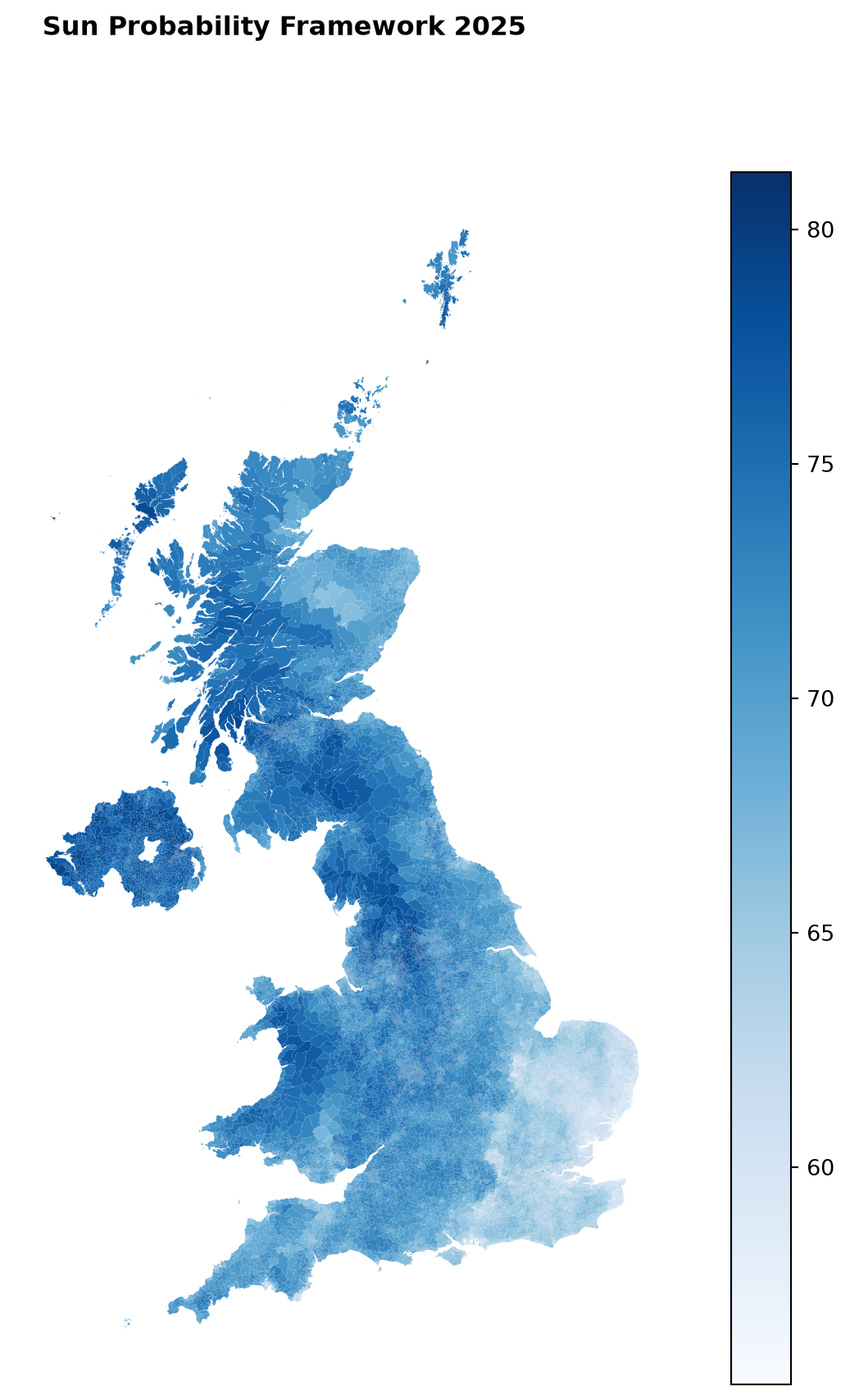
Note
The spatial pattern broadly reflects well-known UK climatology. Higher SPF values (greater cloud probability) are generally observed in Scotland, Wales, and the north and west of Britain, where cloud cover tends to be more persistent, while lower SPF values (clearer conditions) are more common across southern and eastern England. This provides useful context before examining how conditions changed between 2024 and 2025.
Preparing the Data
To compare the two years, we first rename the SPF variable before joining both datasets using their common small-area identifier.
spf_24 = spf_24.rename(columns={"cloud_probability": "spf_2024"})

spf_25 = spf_25.rename(columns={"cloud_probability": "spf_2025"})

spf = spf_24.merge(
    spf_25[
        [
            "data_zone_code",
            "spf_2025",
        ]
    ],
    on="data_zone_code",
)

spf.head()| data_zone_code | spf_2024 | geometry | spf_2025 | |
|---|---|---|---|---|
| 0 | E01000001 | 75.3732 | MULTIPOLYGON (((532105.312 182010.574, 532162.... | 65.8183 |
| 1 | E01000002 | 76.4528 | MULTIPOLYGON (((532634.497 181926.016, 532619.... | 65.0145 |
| 2 | E01000003 | 75.7094 | MULTIPOLYGON (((532135.138 182198.131, 532158.... | 67.9649 |
| 3 | E01000005 | 77.1327 | MULTIPOLYGON (((533808.018 180767.774, 533649.... | 64.9263 |
| 4 | E01000006 | 77.5409 | MULTIPOLYGON (((545122.049 184314.931, 545271.... | 65.9036 |
Calculating Annual Change
The difference between the two years provides a simple measure of how cloud cover conditions changed.
Positive values indicate higher SPF (more cloud) in 2025, while negative values indicate lower SPF (less cloud, clearer conditions) in 2025 relative to 2024.
spf["change"] = spf["spf_2025"] - spf["spf_2024"]

spf["percent_change"] = 100 * spf["change"] / spf["spf_2024"]
Summary Statistics
Before exploring the spatial patterns, it is useful to summarise the overall national changes.
print(f"Average SPF 2024: {spf['spf_2024'].mean():.1f}")
print(f"Average SPF 2025: {spf['spf_2025'].mean():.1f}")

print(f"Mean change: {spf['change'].mean():.1f}")
print(f"Median change: {spf['change'].median():.1f}")

print(f"Maximum increase: {spf['change'].max():.1f}")
print(f"Maximum decrease: {spf['change'].min():.1f}")
Average SPF 2024: 78.2
Average SPF 2025: 70.9
Mean change: -7.3
Median change: -7.3
Maximum increase: 5.9
Maximum decrease: -20.9
Note
The average SPF declined between 2024 and 2025, indicating a fall in average cloud probability — in other words, conditions were on average clearer and sunnier in 2025 than in 2024. However, these summary statistics do not reveal whether the change occurred uniformly across the country, which is explored in the following sections.
Distribution of Annual Change
National averages can hide substantial local variation. A histogram allows us to see whether most small areas experienced similar changes or whether only a small number changed substantially.
Freedman-Diaconis
Before plotting the distribution, we estimate an appropriate number of histogram bins using the Freedman–Diaconis rule. This method adapts the bin width according to both the number of observations and the variability of the data, helping to reveal the underlying distribution without choosing an arbitrary number of bins.
# Freedman-Diaconis Calculations
data = spf["change"]
data_points = len(data)
q1 = data.quantile(0.25)
q3 = data.quantile(0.75)

# Calculate interquartile range
iqr = q3 - q1

bin_width = (2 * iqr) / (data_points ** (1 / 3))

spf_change_bins = int(np.ceil((data.max() - data.min()) / bin_width))
spf_change_bins = round(spf_change_bins, 0)
print(f"Amount of SPF bins: {spf_change_bins}")
Amount of SPF bins: 98from scipy.stats import gaussian_kde
fig, ax = plt.subplots(figsize=(8, 5))
spf["change"].plot(
kind="hist",
color="darkslategrey",
bins=spf_change_bins,
density=True,
alpha=0.6,
ax=ax,
)
# KDE overlay -- smooths the histogram into a continuous density curve,
# making it easier to see whether the double-peak is a real feature
# or just an artefact of the bin edges
kde = gaussian_kde(spf["change"].dropna())
x_range = np.linspace(spf["change"].min(), spf["change"].max(), 500)
ax.plot(x_range, kde(x_range), color="firebrick", linewidth=2)
ax.set_xlabel("Change in SPF")
ax.set_ylabel("Density")
plt.tight_layout()
plt.title("Distribution of Sun Probability Framework Change, United Kingdom")
plt.show()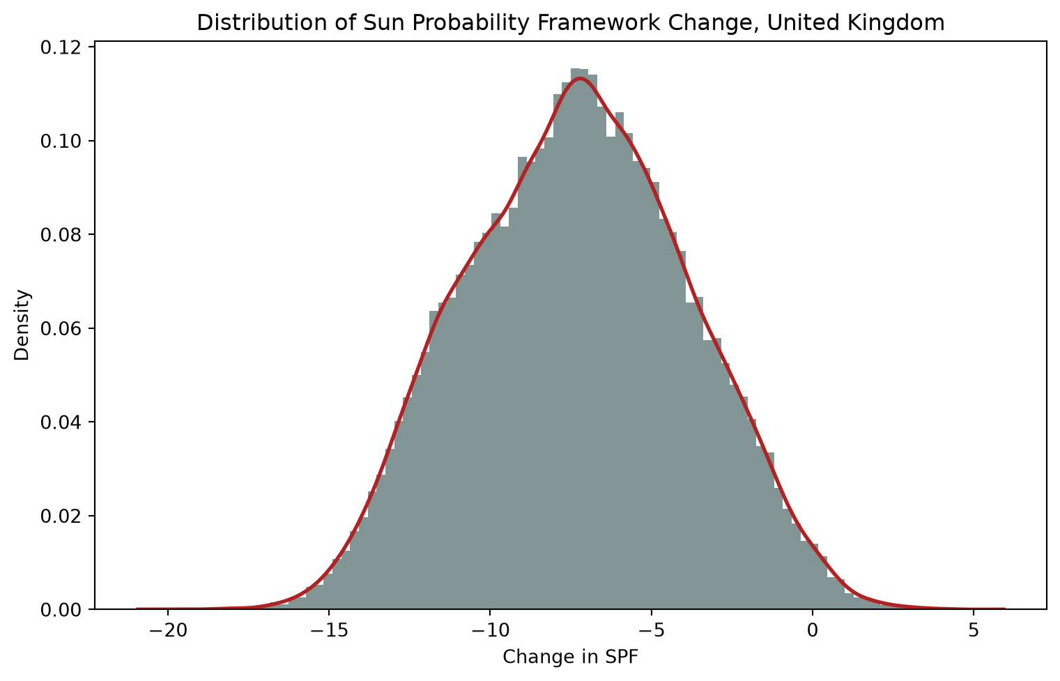
The distribution is approximately bell shaped and clearly centred well below zero rather than around it. This indicates that most small areas experienced lower SPF values in 2025 than in 2024, showing a fall in cloud probability, and so generally clearer conditions across much of the United Kingdom during 2025. The bulk of the distribution falls between roughly −5 and −10 SPF units, with the peak around −7. Although a small number of areas recorded increases in SPF (i.e. became cloudier), these are comparatively rare and confined to a thin tail above zero.
Mapping Annual Change
Mapping the changes allows us to investigate whether increases and decreases occur randomly or form larger geographical patterns.
norm = TwoSlopeNorm(
    vmin=spf["change"].min(),
    vcenter=0,
    vmax=spf["change"].max(),
)

fig, ax = plt.subplots(figsize=(8, 10))

spf.plot(
    column="change",
    cmap="RdBu",
    norm=norm,
    legend=True,
    ax=ax,
)

ax.set_title(
    "Change in Sun Probability Framework (2024-2025)",
    fontweight="bold",
)

ax.axis("off")

plt.tight_layout()
plt.show()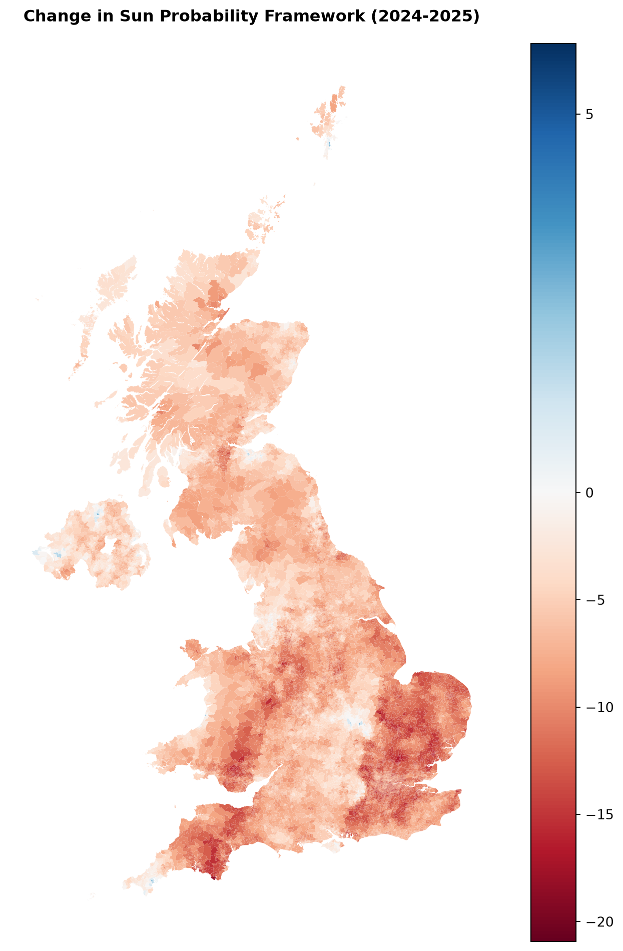
Note
Although most of the United Kingdom experienced a fall in SPF (clearer conditions) in 2025, the magnitude of change varies considerably across space. The largest falls are concentrated in the South East, the South West (including Cornwall), and parts of West Wales, where SPF dropped by 15–20 points in places. Central England shows a more moderate, though still substantial, fall.
By contrast, Scotland and Northern Ireland show barely any change at all — much of both nations sits close to white on the map, with only a few scattered patches of a slight increase (cloudier conditions) in the far north of Scotland. Rather than occurring randomly, the changes form a clear geographical gradient running roughly south-east to north-west, suggesting that differences in regional weather systems influenced cloud cover during the year.
Largest Increases & Decreases
We can identify the small areas experiencing the largest increases and decreases in SPF, allowing us to see specifically which areas are changing the most.
top = spf.sort_values("change", ascending=False).head(20)
bottom = spf.sort_values("change").head(20)

fig, ax = plt.subplots(figsize=(8, 10))

spf.plot(
    color="lightgrey",
    edgecolor="white",
    linewidth=0.1,
    ax=ax,
)

# Plot as markers at each polygon's centroid
top_centroids = top.geometry.centroid
bottom_centroids = bottom.geometry.centroid

ax.scatter(
    top_centroids.x,
    top_centroids.y,
    color="#2166ac",
    s=60,
    edgecolor="black",
    linewidth=0.5,
    zorder=3,
    label="Largest increase (top 20)",
)

ax.scatter(
    bottom_centroids.x,
    bottom_centroids.y,
    color="#b2182b",
    s=60,
    edgecolor="black",
    linewidth=0.5,
    zorder=3,
    label="Largest decrease (bottom 20)",
)

ax.set_title(
    "Small Areas with the Largest SPF Increases and Decreases (2024-2025)",
    fontweight="bold",
)

ax.axis("off")
ax.legend(loc="lower left", frameon=True, fontsize=9)

plt.tight_layout()
plt.show()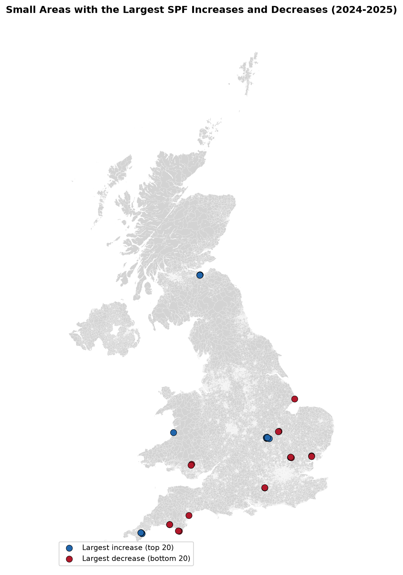
While national maps reveal broad geographical patterns, ranking and mapping individual small areas lets us pinpoint exactly where the most extreme changes occurred, rather than only where change was typical. These specific areas — visible as the highlighted markers above — would be a natural starting point for further investigation into what drove such large shifts.
Overall Direction of Change
increase = (spf["change"] > 0).sum()
decrease = (spf["change"] < 0).sum()
unchanged = (spf["change"] == 0).sum()

total = len(spf)

print(f"Increased SPF: {increase:,} ({100*increase/total:.1f}%)")
print(f"Decreased SPF: {decrease:,} ({100*decrease/total:.1f}%)")
print(f"No change: {unchanged:,} ({100*unchanged/total:.1f}%)")
Increased SPF: 609 (1.3%)
Decreased SPF: 46,235 (98.7%)
No change: 0 (0.0%)
Note
Almost every small area recorded a fall in SPF between 2024 and 2025, demonstrating that this was not driven by a handful of extreme locations but represented a widespread national pattern. While the magnitude of change varied spatially, the overall picture is one of generally clearer, less cloudy conditions during 2025.
What Have We Learnt?
In this notebook we have:
- introduced the Sun Probability Framework (SPF) product
- explored the spatial distribution of SPF across the United Kingdom
- compared annual SPF values between 2024 and 2025
- quantified national changes using summary statistics
- examined the distribution of annual change using the Freedman–Diaconis rule
- mapped where cloud cover conditions increased and decreased
- identified the small areas experiencing the largest increases and decreases in SPF
This notebook demonstrates how annual SPF products can be used to investigate changes in cloud cover conditions over time. In the next case study, the SPF product will be combined with socioeconomic data to explore how differences in cloud cover conditions relate to broader geographical and social questions.
Footnotes
“Small area” refers to the finest commonly used statistical geography in each UK nation: Lower Layer Super Output Areas (LSOAs) in England and Wales, Data Zones in Scotland, and Super Output Areas (SOAs) in Northern Ireland. These are harmonised under a single
data_zone_codeidentifier in the Imago datasets.↩︎Burchell, K., Rhodes, L.E. and Webb, A.R. (2020) ‘Public Awareness and Behaviour in Great Britain in the Context of Sunlight Exposure and Vitamin D’, International Journal of Environmental Research and Public Health, 17(18), 6924.↩︎
Fleming, D., Grimes, A., Lebreton, L., Maré, D.C. and Nunns, P. (2018) ‘Valuing sunshine’, Regional Science and Urban Economics, 68, pp. 268–276.↩︎
Hollis, D., McCarthy, M., Kendon, M., Legg, T. and Simpson, I. (2019) ‘HadUK-Grid—A new UK dataset of gridded climate observations’, Geoscience Data Journal, 6(2), pp. 151–159.↩︎