Precipitation - Annual Rainfall vs. Anomalies

Goal: Using the Imago MSOA Precipitation Product, we compare annual rainfall totals with long-term rainfall anomalies to investigate whether the wettest locations in 2024 were also the locations that departed furthest from their historical rainfall patterns.

Data:

Precipitation per MSOA 2024

A question for the data

In the previous case studies, we explored where UK rainfall was concentrated and how seasonal patterns drove annual totals. However, a high annual total does not necessarily mean a region’s rainfall deviated from its long-term historical baseline.

Some parts of the UK are consistently wet and regularly receive large amounts of rainfall. Other areas are typically much drier and may appear unremarkable in annual rainfall rankings while still experiencing an exceptionally unusual year.

To investigate this, we compare annual rainfall totals against anomalies derived from a long-term climatological baseline, as well as the frequency of extreme daily rainfall events.

Installing Libraries

Python

# Geospatial Libraries
import pandas as pd
import geopandas as gpd
import numpy as np

# Plotting
import matplotlib.pyplot as plt

Loading the Data

Using geopandas, we read the gpkg directly as it contains both the boundary and the rainfall data.

Python

precip_msoa = gpd.read_file("data/precipitation_indicators_MSOA_2024.gpkg")
precip_msoa.head()

	dt_zn_c	dt_zn_n	rainfall_annual_mm	winter_rainfall	spring_rainfall	summer_rainfall	autumn_rainfall	annual_anomaly_abs	annual_anomaly_std	extreme_days_4sd	year	geometry
0	E02000001	City of London 001	696.647095	223.671677	189.220276	107.580292	218.248856	158.290131	2.148560	26.304880	2024	MULTIPOLYGON (((532135.138 182198.131, 532158....
1	E02000002	Barking and Dagenham 001	695.338257	236.243835	192.781601	106.833694	205.600983	131.554367	1.715453	23.520077	2024	MULTIPOLYGON (((548881.563 190845.265, 548881....
2	E02000003	Barking and Dagenham 002	667.498779	230.828064	185.345505	100.507462	195.728653	120.716499	1.595210	22.027685	2024	MULTIPOLYGON (((549102.438 189324.625, 548954....
3	E02000004	Barking and Dagenham 003	611.439758	218.056824	171.161316	89.372581	175.921600	93.010658	1.238803	23.146259	2024	MULTIPOLYGON (((551550.056 187364.705, 551478 ...
4	E02000005	Barking and Dagenham 004	632.301819	224.054337	176.073090	93.059616	183.112747	102.117798	1.371893	22.568747	2024	MULTIPOLYGON (((549099.634 187656.076, 549161....

For this case study we will be using four of the variables:

rainfall_annual_mm: Total annual rainfall in millimetres.
annual_anomaly_abs: The absolute annual precipitation anomaly from historical baseline in mm (so it is actual - expected).
annual_anomaly_std: Standardised rainfall anomaly relative to historical variability (in standard deviations).
extreme_days_4sd: number of days where daily rainfall exceeded 4 standard deviations above historical daily mean.

Note

The two anomaly measures describe different aspects of unusual rainfall.

annual_anomaly_abs tells us how much wetter or drier conditions were than expected (in mm). annual_anomaly_std tells us how unusual that difference was relative to the normal variability experienced in that location (in standard deviations).

A large absolute anomaly does not necessarily imply a large standardised anomaly, and vice a versa.

extreme_days_4sd identifies unusually intense rainfall events rather than the general wetness. It is possible that a location may receive high annual rainfall, but very few or no extreme days. Conversely, an area with modest annual rainfall might receive the majority of its precipitation during just a few intense storm events.

Summary Statistics

Before mapping the data, it is useful to understand the whole range of values.

Python

precip_msoa[
    [
        "rainfall_annual_mm",
        "annual_anomaly_abs",
        "annual_anomaly_std",
        "extreme_days_4sd",
    ]
].agg(["mean", "std", "min", "max"])

	rainfall_annual_mm	annual_anomaly_abs	annual_anomaly_std	extreme_days_4sd
mean	972.689669	218.666213	2.071002	25.435176
std	274.112145	135.570063	1.169335	6.249295
min	516.364502	-183.354797	-1.736415	3.339783
max	3140.853516	963.079346	6.566710	44.779831

Mapping Annual Rainfall

To begin, let’s remind ourselves of what the annual rainfall looks like across the country so we have a clear baseline for comparison.

Python

p01 = precip_msoa["rainfall_annual_mm"].quantile(0.01)
p99 = precip_msoa["rainfall_annual_mm"].quantile(0.99)

fig, ax = plt.subplots(figsize=(8, 8))

precip_msoa.plot(
    column="rainfall_annual_mm",
    cmap="Blues",
    legend=True,
    linewidth=0,
    ax=ax,
    vmin=p01,
    vmax=p99,
)

ax.set_title("Annual Rainfall Across MSOAs, 2024", fontweight="bold")
ax.set_axis_off()
plt.tight_layout()
plt.show()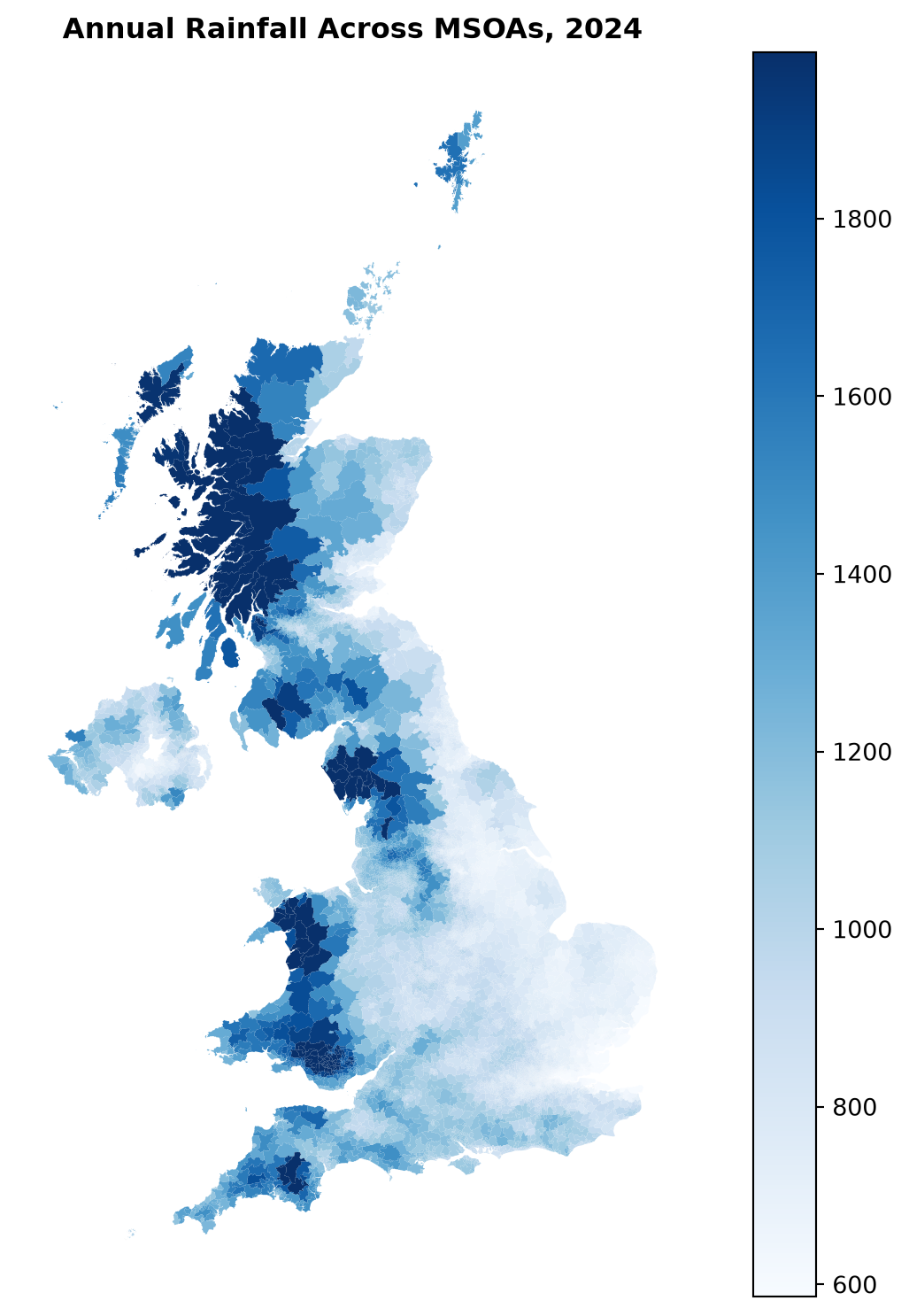

Mapping Standardised Rainfall Anomalies

Standardised anomalies account for local variability and therefore provide a clearer indication of how unusual conditions were. By comparing this map with the total rainfall plot, we can visually identify regions where the climate anomalies did not align with absolute rainfall totals.

Python

p01 = precip_msoa["annual_anomaly_std"].quantile(0.01)
p99 = precip_msoa["annual_anomaly_std"].quantile(0.99)

limit = max(abs(p01), abs(p99))

fig, ax = plt.subplots(figsize=(8, 8))

precip_msoa.plot(
    column="annual_anomaly_std",
    cmap="RdBu",
    legend=True,
    linewidth=0,
    ax=ax,
    vmin=-limit,
    vmax=limit,
)

ax.set_title("Standardised Rainfall Anomaly, 2024", fontweight="bold")
ax.set_axis_off()
plt.tight_layout()
plt.show()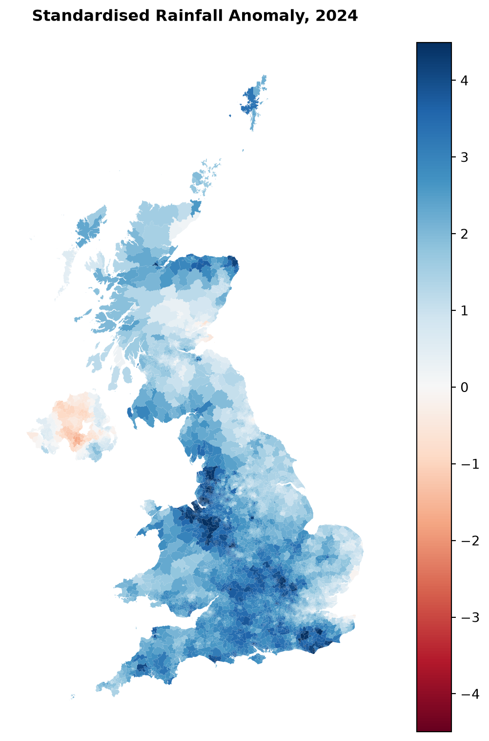

Note

The anomaly maps differ noticeably from the annual rainfall map. The wettest parts of the UK are not automatically the most anomalous. While you can see that there is overlap with parts of the country, some parts which have large rainfall totals show modest anomalies while those with much lower total rainfalls (such as south England) are having fairly strong anomalies. Most interesting is Northern Ireland, which was the only major region to record negative anomalies, indicating it was drier than its historical average.

This shows why rainfall totals and rainfall anomalies are answering different questions.

Does high annual rainfall imply unusual climatic conditions?

To investigate the relationship directly, we compare annual rainfall against standardised anomaly values.

Python

fig, ax = plt.subplots(figsize=(7, 6))

ax.scatter(
    precip_msoa["rainfall_annual_mm"], precip_msoa["annual_anomaly_std"], alpha=0.5, s=2
)
ax.axhline(
    0,
    color="red",
    linestyle="--",
    linewidth=1,
    label="Baseline (Mean)",
)
x = precip_msoa["rainfall_annual_mm"]
y = precip_msoa["annual_anomaly_std"]
m, c = np.polyfit(x, y, 1)
ax.plot(
    x,
    m * x + c,
    color="darkslategrey",
    linewidth=2,
    alpha=0.8,
    label=f"Trend (slope: {m:.4f})",
)

ax.set_xlabel("Annual Rainfall (mm)")
ax.set_ylabel("Standardised Anomaly")
ax.set_title("Annual Rainfall vs Standardised Anomaly", fontweight="bold")
ax.grid(linestyle="--", alpha=0.3)

plt.tight_layout()
plt.show()

corr = precip_msoa[["rainfall_annual_mm", "annual_anomaly_std"]].corr().iloc[0, 1]

print(f"Correlation: {corr:.2f}")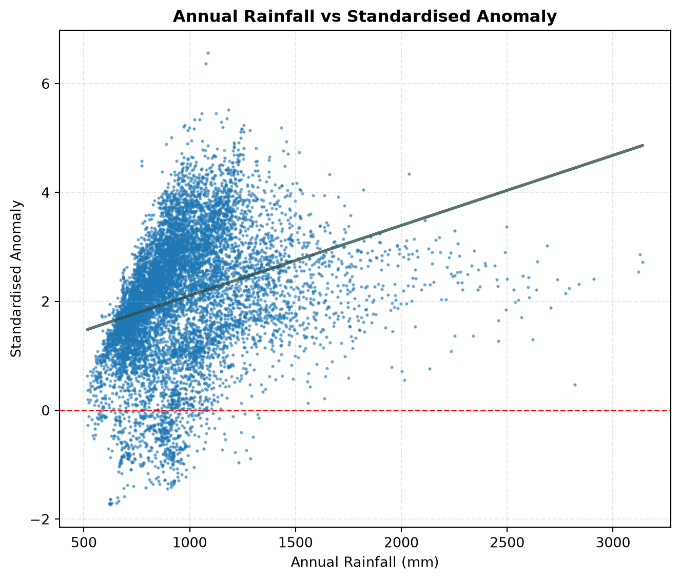

Correlation: 0.30

Note

If wet places were also always the most unusual places, we would expect a strong positive relationship between annual rainfall and standardised anomaly.

Despite this, we actually have a weak to moderate correlation of r = 0.3 and a scatter graph which shows a much more complex relationship. For one, the vast majority of MSOAs experienced a positively anomalous year, suggesting as a whole 2024 was a wet year for the UK. The most extreme MSOAs, especially the two 6+ standard deviations, are actually very normal MSOAs for total rainfall. Meanwhile, the MSOA with the highest absolute rainfall (roughly 2,800 mm) had a standardised anomaly of nearly zero, meaning this high total was typical for the area.

This reinforces the distinction between rainfall amount and rainfall unusuality and how the total rainfall doesn’t define anomalous rainfall.

Locating the Most Anomalous Places

As the wettest places and the most anomalous places are not the same, we next identify the specific locations behind these extremes.

Python

most_anomalous = precip_msoa.nlargest(10, "annual_anomaly_std")[
    ["dt_zn_c", "dt_zn_n", "annual_anomaly_std"]
]

least_anomalous = precip_msoa.nsmallest(10, "annual_anomaly_std")[
    ["dt_zn_c", "dt_zn_n", "annual_anomaly_std"]
]

print("Highest anomalies:")
print(most_anomalous.to_string(index=False))

print("\nLowest anomalies:")
print(least_anomalous.to_string(index=False))

Highest anomalies:
  dt_zn_c            dt_zn_n  annual_anomaly_std
E02004698 East Hampshire 002            6.566710
E02004699 East Hampshire 003            6.364801
W02000073     Flintshire 016            5.520726
E02001480         Wirral 014            5.457350
W02000055   Denbighshire 014            5.452836
W02000071     Flintshire 014            5.359298
E02001492         Wirral 026            5.344003
E02006030     Shropshire 016            5.342445
E02004381          Lewes 003            5.292243
E02004401         Rother 010            5.239768

Lowest anomalies:
  dt_zn_c     dt_zn_n  annual_anomaly_std
N21000068    Armagh_A           -1.736415
N21000071    Armagh_D           -1.716482
N21000070    Armagh_C           -1.716361
N21000069    Armagh_B           -1.715640
N21000073    Armagh_F           -1.714733
N21000074    Armagh_G           -1.708549
N21000075    Armagh_H           -1.700482
N21000684 Dungannon_J           -1.672115
N21000151    Cusher_B           -1.642871
N21000087 Portadown_J           -1.632483

Comparing these rankings to the absolute rainfall list highlights a clear divergence. Although Scotland dominated absolute totals, it has no MSOAs in the top 10 highest anomalies, which are instead occupied by English and Welsh locations. On the other end, the ten lowest anomalies are concentrated entirely in Northern Ireland, specifically in County Armagh and neighbouring County Tyrone. While Armagh is typically a drier part of Northern Ireland, in 2024 it was unusually dry even by its own historical standards.

To clearly visualise where these MSOAs are, we can quickly map them so it highlights solely those MSOAs.

Python

target_msoas = pd.concat([most_anomalous, least_anomalous])

colors = target_msoas["annual_anomaly_std"].apply(lambda x: "blue" if x >= 0 else "red")
target_msoas["plot_color"] = colors

fig, ax = plt.subplots(figsize= (7,7))

precip_msoa.plot(
    ax=ax,
    color="gainsboro",
    edgecolor="none",
    linewidth=0.3,
)
highlighted_gdf = precip_msoa[
    precip_msoa["dt_zn_c"].isin(target_msoas["dt_zn_c"])
].copy()
highlighted_gdf = highlighted_gdf.merge(
    target_msoas[["dt_zn_c", "plot_color"]], on="dt_zn_c"
)
highlighted_gdf.plot(
    ax=ax,
    color=highlighted_gdf["plot_color"],
    linewidth=0.8,
)

ax.set_title(
    "Top 10 Most and Least Anomalous MSOAs\n(Blue = Positive, Red = Negative)",
    fontsize=14,
)
ax.axis("off")
plt.show()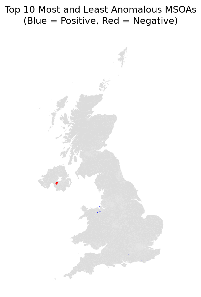

Understanding How Unusual Rainfall Occurred

Knowing that an area experienced an unusually wet year still leaves an important question unanswered.

An MSOA may have accumulated an unusually large annual rainfall total because rainfall was consistently above average throughout the year, or because a small number of very intense rainfall events contributed a large proportion of the annual total.

The extreme_days_4sd indicator allows us to investigate this by counting the number of days where rainfall exceeded four standard deviations above the historical daily mean.

If areas with the highest rainfall anomalies also experienced many extreme rainfall days, this would suggest that intense rainfall events played an important role in producing those unusually wet conditions.

Python

p01 = precip_msoa["extreme_days_4sd"].quantile(0.01)
p99 = precip_msoa["extreme_days_4sd"].quantile(0.99)

fig, ax = plt.subplots(figsize=(8, 8))

precip_msoa.plot(
    column="extreme_days_4sd",
    cmap="Blues",
    linewidth=0,
    legend=True,
    ax=ax,
    vmin=p01,
    vmax=p99,
)

ax.set_title("Extreme Rainfall Days Across MSOAs, 2024", fontweight="bold")
ax.set_axis_off()

plt.tight_layout()
plt.show()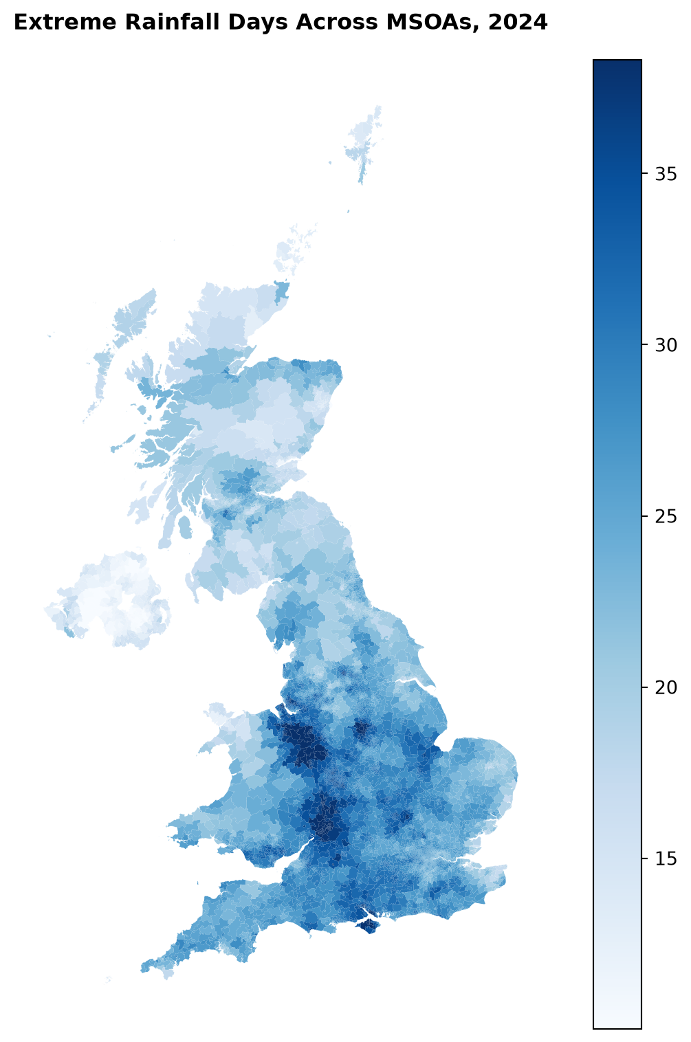

The geographic pattern of extreme rainfall is concentrated much further west than annual rainfall or anomalies.

While some high-rainfall areas recorded many extreme days, others accumulated large totals with very few extreme events. Similarly, some moderate-rainfall areas saw unusually high counts of extreme days. Notably, the Welsh Marches stands out with a high concentration of extreme days.

This shows that annual totals can be driven by completely different rainfall regimes.

Annual Rainfall and Extreme Rainfall Days

While the maps provide a useful visual comparison, we can investigate the relationship directly by comparing annual rainfall against the number of extreme rainfall days.

Python

fig, ax = plt.subplots(figsize=(7, 6))

ax.scatter(
    precip_msoa["rainfall_annual_mm"], precip_msoa["extreme_days_4sd"], alpha=0.4
)

m, c = np.polyfit(
    precip_msoa["rainfall_annual_mm"],
    precip_msoa["extreme_days_4sd"],
    1,
)

ax.plot(
    precip_msoa["rainfall_annual_mm"],
    m * precip_msoa["rainfall_annual_mm"] + c,
    color="darkslategrey",
    linewidth=2,
)

ax.set_xlabel("Annual Rainfall (mm)")
ax.set_ylabel("Extreme Rainfall Days")

ax.set_title("Annual Rainfall vs Extreme Rainfall Days", fontweight="bold")

ax.grid(alpha=0.3)

plt.tight_layout()
plt.show()

corr = precip_msoa[["rainfall_annual_mm", "extreme_days_4sd"]].corr().iloc[0, 1]

print(f"Correlation: {corr:.2f}")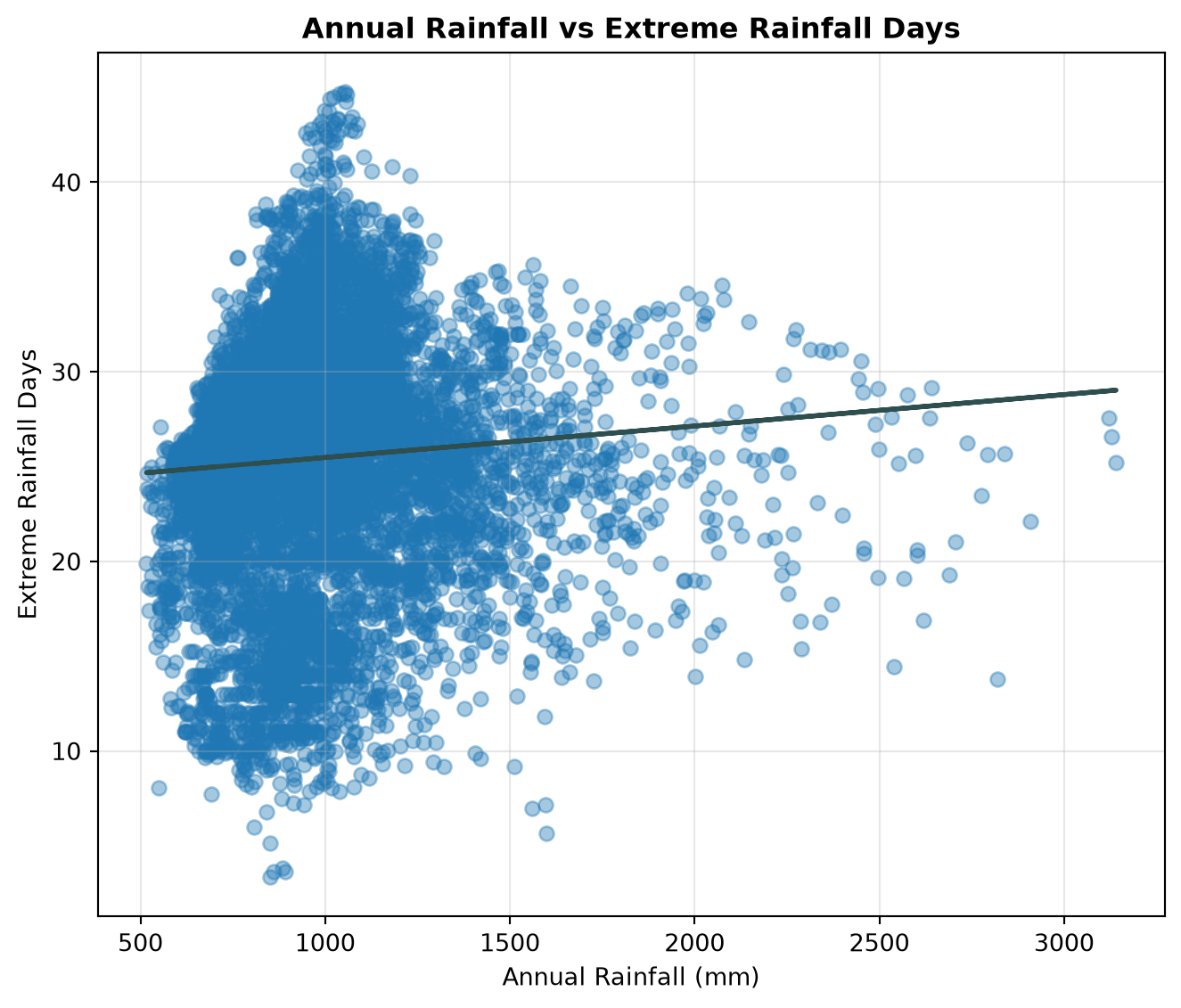

Correlation: 0.07

If annual rainfall was driven by extreme rainfall events, we would expect MSOAs with higher annual rainfall totals to also experience substantially more extreme rainfall days. Instead, the relationship is virtually absent, as shown by a weak correlation of 0.07.

While there is a very slight positive trend, the spread oif points shows that locations with similar annual rainfall totals can experience very different numbers of extreme rainfall days. Likewise, some relatively dry locations experience just as many extreme rainfall days as much wetter areas.

This suggests that annual rainfall and rainfall extremity capture different characteristics of the UK’s climate. High annual rainfall does not necessarily imply that rainfall occurred through unusually intense events.

Extreme Rainfall Relative to Total Rainfall

Python

m, c = np.polyfit(
    precip_msoa["rainfall_annual_mm"],
    precip_msoa["extreme_days_4sd"],
    1,
)

precip_msoa["expected_extreme_days"] = m * precip_msoa["rainfall_annual_mm"] + c

precip_msoa["extreme_day_residual"] = (
    precip_msoa["extreme_days_4sd"] - precip_msoa["expected_extreme_days"]
)

# Symmetric colour scale
p01 = precip_msoa["extreme_day_residual"].quantile(0.01)
p99 = precip_msoa["extreme_day_residual"].quantile(0.99)

limit = max(abs(p01), abs(p99))

fig, ax = plt.subplots(figsize=(8, 8))

precip_msoa.plot(
    column="extreme_day_residual",
    cmap="RdBu",
    linewidth=0,
    legend=True,
    ax=ax,
    vmin=-limit,
    vmax=limit,
    legend_kwds={
        "label": "Extreme rainfall days relative to expectation",
        "shrink": 0.6,
    },
)

ax.set_title(
    "Extreme Rainfall Days Relative to Annual Rainfall",
    fontweight="bold",
)

ax.set_axis_off()

plt.tight_layout()
plt.show()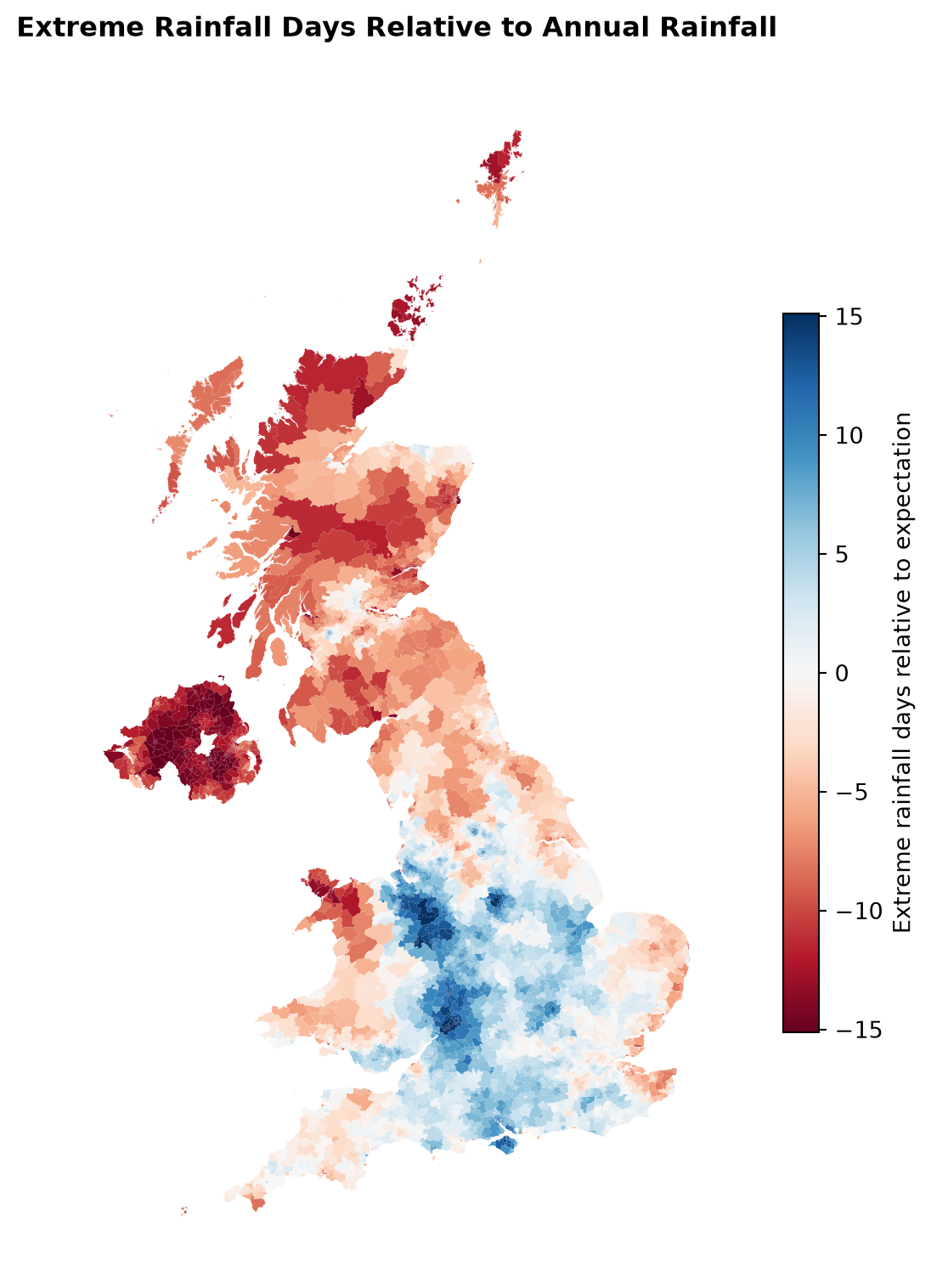

Note

Although annual rainfall and extreme rainfall days show almost no overall statistical relationship, distinct spatial patterns are still visible when mapped.

By comparing the number of extreme days to the expected amount of annual rainfall for each MSOA, we can identify locations where rainfall was disproportionately concentrated in extreme events. The clearest example is Northern Ireland; across the vast majority of its six counties, regions receive substantial annual rainfall with relatively few extreme days, suggesting that precipitation is distributed in smaller, more consistent amounts throughout the year. Although less pronounced, a similar pattern appears in North Wales and Scotland, which also record more rainfall relative to their extreme days.

Conversely, the Welsh Marches—and to some extent central and southern England—exhibit the opposite pattern, experiencing a higher number of extreme days than expected based on their annual rainfall totals. This demonstrates that even in the absence of a strong statistical correlation, mapping can reveal meaningful geographical trends in how rainfall is delivered.

What have we learnt?

Throughout this notebook we investigated whether the wettest places in the UK were also the most unusual and whether unusually wet conditions were associated with more extreme rainfall events.

The analysis suggests that neither assumption consistently holds.

The wettest MSOAs are not automatically the most anomalous relative to their historical climate, demonstrating why anomaly measures provide important context beyond annual rainfall totals. Similarly, annual rainfall and extreme rainfall days show almost no overall relationship, indicating that total rainfall alone cannot explain how rainfall was experienced.