# Core data handling and plotting
library(tidyverse)   # Data manipulation + ggplot2
library(readxl)      # Reading Excel files (IMD)

# Spatial data and mapping
library(sf)          # Simple Features

# Regression
library(fixest)      # Fast OLS / fixed-effects models

# Python interop (only needed if rendering both languages)
library(reticulate)Air temperature - Basics
Goal: Use the Imago air temperature product to explore the relationship between heat exposure and deprivation in England. We start by exploring a cross-section.
Training approach: The instructor demonstrates the workflow end-to-end. We use just two indicators throughout — summer_max_tmp and extreme_hot_days_mean — but the same logic transfers to any of the sixteen indicators in the product.
NoteGetting the data
The Imago air temperature data is hosted on our data catalogue. To download it:
- Sign up for a free account on the data catalogue and log in.
- Search for
air temperature MSOA(or browse the temperature datasets). - Open each yearly dataset — for example, Air Temperature Indicators per MSOA in 2015 — and download the
.gpkgfile. - Save the files into a
./data/folder in your project, keeping the original filenames (temperature_indicators_MSOA_2015.gpkg, …,temperature_indicators_MSOA_2024.gpkg).
For this training you’ll need all ten years (2015–2024) if you plan to follow Part 2 onwards. For Part 1 alone, only the 2024 file is needed.
Cross-sectional foundations
We start with a single year. The Imago air temperature product publishes one geopackage per year covering 2015–2024; we use 2024 here as our cross-section. The questions for this sections the natural ones a researcher would ask the first time they meet a new dataset: what does the distribution look like, where in the country are the hottest places, and how does heat exposure relate to deprivation?
Installing packages
We load core packages for working with spatial data, plotting, and regression. See detailed descriptions of R and Python for the geospatial side.
# Standard library
import os
import tempfile
import zipfile

# Data & geospatial
import numpy as np
import pandas as pd
import geopandas as gpd

# Plotting
import matplotlib.pyplot as plt

# Statistics
import statsmodels.formula.api as smf
from scipy import stats

# Networking
import requests
Loading the 2024 cross-section
The Imago air temperature product publishes one geopackage per year. Each file already contains the MSOA boundary geometry alongside the temperature indicators, so we do not need a separate boundary file.
msoa_temp <- read_sf("./data/temperature_indicators_MSOA_2024.gpkg")

# A look at the first few rows
glimpse(msoa_temp)
Rows: 9,448
Columns: 17
$ dt_zn_c <chr> "E02000001", "E02000002", "E02000003", "E0200000…
$ dt_zn_n <chr> "City of London 001", "Barking and Dagenham 001"…
$ annual_mean_tmp <dbl> 12.76346, 12.07690, 12.20336, 12.33897, 12.34112…
$ annual_max_tmp <dbl> 16.28021, 15.99580, 16.07938, 16.19617, 16.16838…
$ annual_min_tmp <dbl> 9.247190, 8.215314, 8.376277, 8.529167, 8.552910…
$ winter_mean_tmp <dbl> 7.962327, 7.301272, 7.425026, 7.562093, 7.556808…
$ spring_mean_tmp <dbl> 12.23706, 11.55152, 11.67148, 11.78149, 11.80289…
$ summer_mean_tmp <dbl> 18.24644, 17.54276, 17.68478, 17.84687, 17.84362…
$ autumn_mean_tmp <dbl> 12.78338, 12.08531, 12.20684, 12.34222, 12.33728…
$ summer_max_tmp <dbl> 23.00629, 22.75395, 22.83498, 22.96780, 22.92410…
$ winter_min_tmp <dbl> 5.307874, 4.413336, 4.557454, 4.709777, 4.712059…
$ temporal_sd_tmp <dbl> 4.218369, 4.201226, 4.209268, 4.221317, 4.220945…
$ tmp_anomaly_absolute <dbl> 2.558206, 2.472255, 2.478608, 2.477158, 2.483515…
$ tmp_anomaly_relative <dbl> 3.939247, 4.046119, 4.044049, 4.074961, 4.043092…
$ extreme_hot_days_mean <dbl> 3.000000, 3.000000, 3.000000, 3.000000, 3.000000…
$ hot_spell_3day_mean <dbl> 7.000000, 7.000000, 7.008710, 8.000000, 7.675590…
$ geom <MULTIPOLYGON [m]> MULTIPOLYGON (((532135.1 18..., MUL…msoa_temp = gpd.read_file("./data/temperature_indicators_MSOA_2024.gpkg")
msoa_temp.head() dt_zn_c ... geometry
0 E02000001 ... MULTIPOLYGON (((532135.138 182198.131, 532158....
1 E02000002 ... MULTIPOLYGON (((548881.563 190845.265, 548881....
2 E02000003 ... MULTIPOLYGON (((549102.438 189324.625, 548954....
3 E02000004 ... MULTIPOLYGON (((551550.056 187364.705, 551478 ...
4 E02000005 ... MULTIPOLYGON (((549099.634 187656.076, 549161....
[5 rows x 17 columns]This file contains all sixteen indicators in the product. For this training we work with two:
summer_max_tmp— the maximum temperature reached during summer, in °C. A central tendency measure of how hot summers get.extreme_hot_days_mean— the mean number of days per year crossing an extreme-heat threshold. An intensity or dose measure of how often heat extremes occur.
These two are conceptually distinct. A place can have moderate summer maxima but many extreme-heat days (a long warm season), or high summer maxima but few extreme days (short, intense peaks). The inequality story may differ between them.
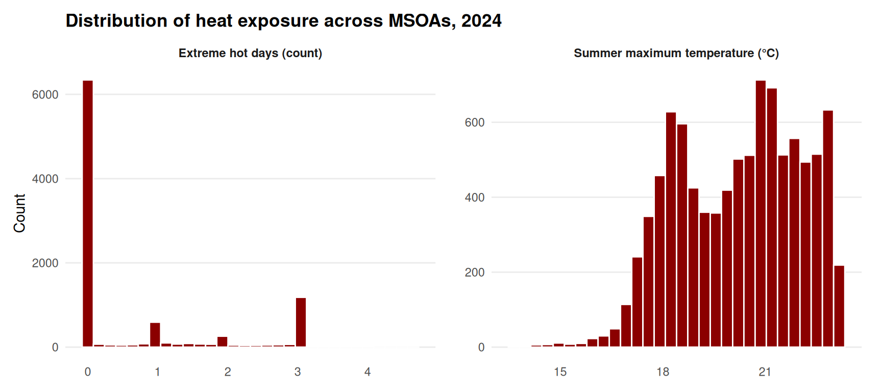
Distribution of the two indicators
We start with summary statistics, then look at the distribution shape with histograms.
msoa_temp %>%
  st_drop_geometry() %>%
  summarise(
    across(
      c(summer_max_tmp, extreme_hot_days_mean),
      list(
        mean = ~mean(.x, na.rm = TRUE),
        sd   = ~sd(.x,   na.rm = TRUE),
        min  = ~min(.x,  na.rm = TRUE),
        max  = ~max(.x,  na.rm = TRUE)
      ),
      .names = "{.col}__{.fn}"
    )
  ) %>%
  pivot_longer(everything(),
               names_to = c("indicator", "stat"),
               names_sep = "__")
# A tibble: 8 × 3
indicator stat value
<chr> <chr> <dbl>
1 summer_max_tmp mean 20.2
2 summer_max_tmp sd 1.80
3 summer_max_tmp min 13.6
4 summer_max_tmp max 23.2
5 extreme_hot_days_mean mean 0.672
6 extreme_hot_days_mean sd 1.11
7 extreme_hot_days_mean min 0
8 extreme_hot_days_mean max 4.65 (
msoa_temp[["summer_max_tmp", "extreme_hot_days_mean"]]
.agg(["mean", "std", "min", "max"])
) summer_max_tmp extreme_hot_days_mean
mean 20.225898 0.672296
std 1.798089 1.110386
min 13.648763 0.000000
max 23.160931 4.648794Now the histograms. We use a small reshape so we can plot both indicators on the same panel grid.
msoa_temp %>%
  st_drop_geometry() %>%
  pivot_longer(
    cols = c(summer_max_tmp, extreme_hot_days_mean),
    names_to  = "indicator",
    values_to = "value"
  ) %>%
  mutate(
    indicator_label = recode(indicator,
      "summer_max_tmp"        = "Summer maximum temperature (°C)",
      "extreme_hot_days_mean" = "Extreme hot days (count)"
    )
  ) %>%
  ggplot(aes(x = value)) +
  geom_histogram(bins = 30, colour = "white", fill = "darkred") +
  facet_wrap(~ indicator_label, scales = "free") +
  labs(
    title = "Distribution of heat exposure across MSOAs, 2024",
    x = NULL, y = "Count"
  ) +
  theme_minimal(base_size = 11) +
  theme(
    plot.title         = element_text(face = "bold", margin = margin(b = 12)),
    strip.text         = element_text(face = "bold", margin = margin(b = 6)),
    panel.grid.minor   = element_blank(),
    panel.grid.major.x = element_blank(),
    panel.spacing.x    = unit(1.5, "lines"),
    plot.margin        = margin(t = 10, r = 15, b = 10, l = 10)
  )
fig, axes = plt.subplots(1, 2, figsize=(11, 4))

axes[0].hist(msoa_temp["summer_max_tmp"].dropna(),
             bins=30, edgecolor="white", color="darkred")
axes[0].set_title("Summer maximum temperature (°C)", fontweight="bold")
axes[0].set_ylabel("Count")

axes[1].hist(msoa_temp["extreme_hot_days_mean"].dropna(),
             bins=30, edgecolor="white", color="darkred")
axes[1].set_title("Extreme hot days (count)", fontweight="bold")
axes[1].set_ylabel("Count")

for ax in axes:
    ax.grid(axis="y", linestyle="--", alpha=0.4)
    ax.grid(axis="x", visible=False)

fig.suptitle("Distribution of heat exposure across MSOAs, 2024",
             fontweight="bold", y=1.02)

plt.tight_layout()
plt.subplots_adjust(wspace=0.25, top=0.88)
plt.show()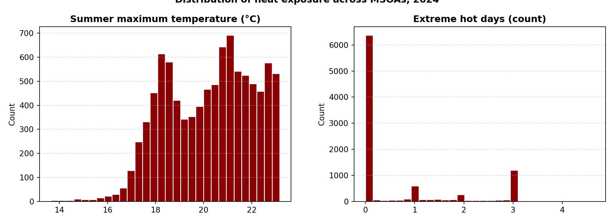
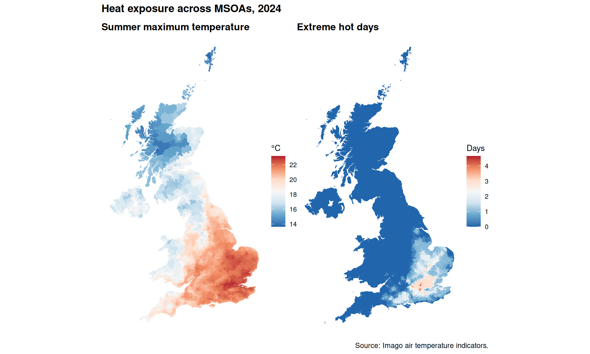
Mapping by local area
Mapping the two indicators side by side gives us the spatial pattern. Hotter and more frequently-extreme MSOAs concentrate in particular regions — predominantly the south-east and major urban areas.
library(patchwork)   # only needed for the side-by-side composite below

map_smt <- ggplot(msoa_temp) +
  geom_sf(aes(fill = summer_max_tmp), colour = NA) +
  scale_fill_distiller(
    palette = "RdBu", direction = -1,
    name = "°C",
    breaks = scales::pretty_breaks(5)
  ) +
  labs(title = "Summer maximum temperature") +
  theme_void(base_size = 10) +
  theme(plot.title = element_text(face = "bold"))

map_ehd <- ggplot(msoa_temp) +
  geom_sf(aes(fill = extreme_hot_days_mean), colour = NA) +
  scale_fill_distiller(
    palette = "RdBu", direction = -1,
    name = "Days",
    breaks = scales::pretty_breaks(5)
  ) +
  labs(title = "Extreme hot days") +
  theme_void(base_size = 10) +
  theme(plot.title = element_text(face = "bold"))

map_smt + map_ehd +
  plot_annotation(
    title = "Heat exposure across MSOAs, 2024",
    caption = "Source: Imago air temperature indicators.",
    theme = theme(plot.title = element_text(face = "bold", size = 13))
  )
fig, axes = plt.subplots(1, 2, figsize=(12, 6))

msoa_temp.plot(
    column="summer_max_tmp", cmap="coolwarm",
    legend=True, ax=axes[0], linewidth=0,
    legend_kwds={"shrink": 0.5, "label": "°C"}
)
axes[0].set_title("Summer maximum temperature", fontweight="bold")
axes[0].set_axis_off()

msoa_temp.plot(
    column="extreme_hot_days_mean", cmap="coolwarm",
    legend=True, ax=axes[1], linewidth=0,
    legend_kwds={"shrink": 0.5, "label": "Days"}
)
axes[1].set_title("Extreme hot days", fontweight="bold")
axes[1].set_axis_off()

fig.suptitle("Heat exposure across MSOAs, 2024", fontweight="bold")
plt.tight_layout()
plt.show()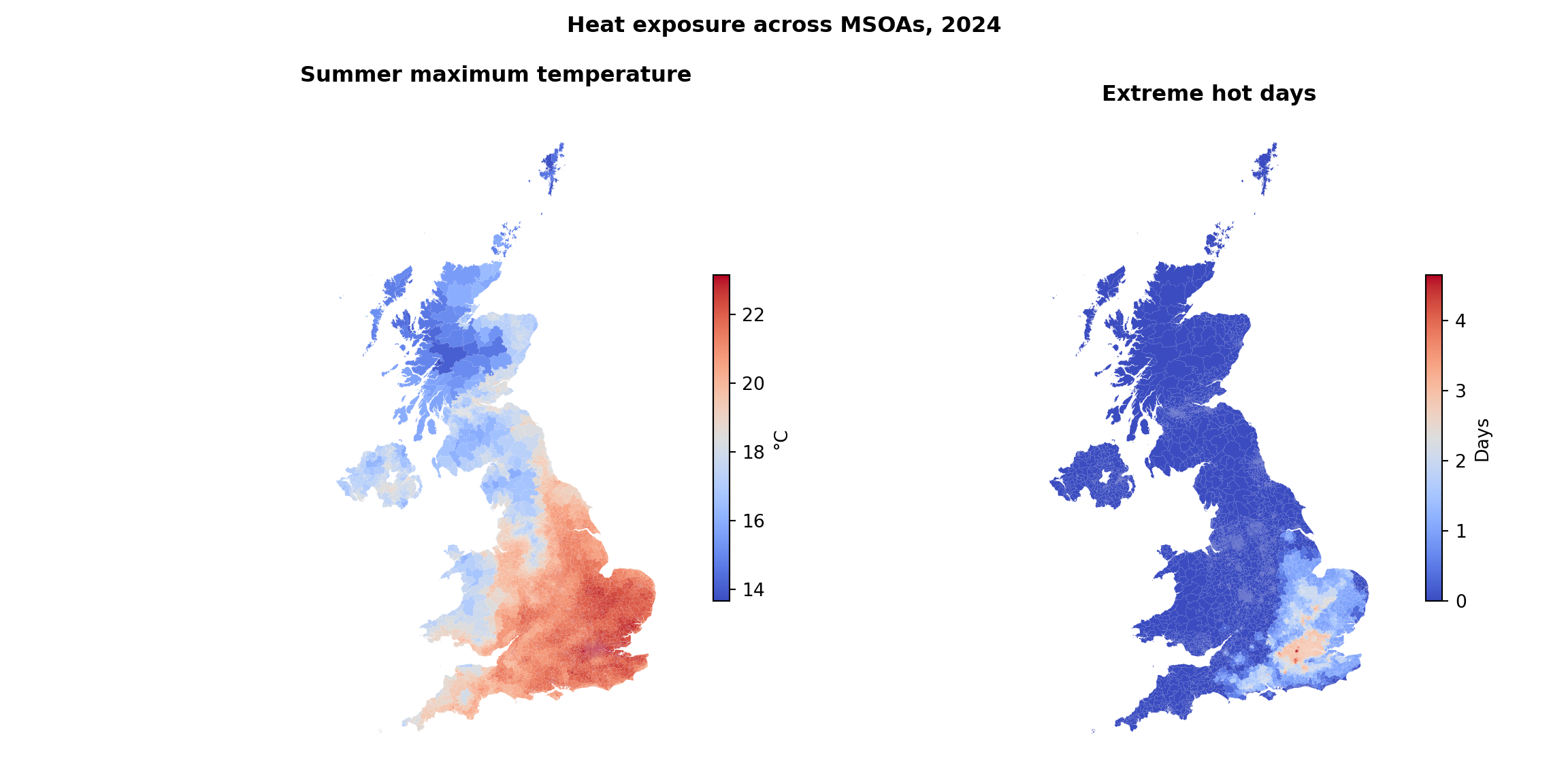
Merge with the Index of Multiple Deprivation
The English Indices of Deprivation 2025 provide the deprivation measure used throughout this training. We focus on the Health Deprivation and Disability domain because heat exposure has a clear pathway through health.
IMD is published at LSOA level; the temperature data are at MSOA level. We therefore need to (i) download IMD, (ii) use the ONS LSOA→MSOA lookup, and (iii) aggregate the LSOA-level health rank up to MSOAs.
Download IMD 2025
tmp_file <- tempfile(fileext = ".xlsx")

download.file(
  url = "https://assets.publishing.service.gov.uk/media/691decfae39a085bda43efcd/File_2_IoD2025_Domains_of_Deprivation.xlsx",
  destfile = tmp_file,
  mode = "wb"
)

imd <- read_excel(tmp_file, sheet = "IoD2025 Domains")
unlink(tmp_file)

names(imd)
[1] "LSOA code (2021)"
[2] "LSOA name (2021)"
[3] "Local Authority District code (2024)"
[4] "Local Authority District name (2024)"
[5] "Index of Multiple Deprivation (IMD) Rank (where 1 is most deprived)"
[6] "Index of Multiple Deprivation (IMD) Decile (where 1 is most deprived 10% of LSOAs)"
[7] "Income Rank (where 1 is most deprived)"
[8] "Income Decile (where 1 is most deprived 10% of LSOAs)"
[9] "Employment Rank (where 1 is most deprived)"
[10] "Employment Decile (where 1 is most deprived 10% of LSOAs)"
[11] "Education, Skills and Training Rank (where 1 is most deprived)"
[12] "Education, Skills and Training Decile (where 1 is most deprived 10% of LSOAs)"
[13] "Health Deprivation and Disability Rank (where 1 is most deprived)"
[14] "Health Deprivation and Disability Decile (where 1 is most deprived 10% of LSOAs)"
[15] "Crime Rank (where 1 is most deprived)"
[16] "Crime Decile (where 1 is most deprived 10% of LSOAs)"
[17] "Barriers to Housing and Services Rank (where 1 is most deprived)"
[18] "Barriers to Housing and Services Decile (where 1 is most deprived 10% of LSOAs)"
[19] "Living Environment Rank (where 1 is most deprived)"
[20] "Living Environment Decile (where 1 is most deprived 10% of LSOAs)" tmp_file = tempfile.NamedTemporaryFile(delete=False, suffix=".xlsx").name
url = ("https://assets.publishing.service.gov.uk/media/"
"691decfae39a085bda43efcd/File_2_IoD2025_Domains_of_Deprivation.xlsx")
r = requests.get(url)
with open(tmp_file, "wb") as f:
f.write(r.content)4337372imd = pd.read_excel(tmp_file, sheet_name="IoD2025 Domains")
os.remove(tmp_file)
print(imd.columns.tolist())['LSOA code (2021)', 'LSOA name (2021)', 'Local Authority District code (2024)', 'Local Authority District name (2024)', 'Index of Multiple Deprivation (IMD) Rank (where 1 is most deprived)', 'Index of Multiple Deprivation (IMD) Decile (where 1 is most deprived 10% of LSOAs)', 'Income Rank (where 1 is most deprived)', 'Income Decile (where 1 is most deprived 10% of LSOAs)', 'Employment Rank (where 1 is most deprived)', 'Employment Decile (where 1 is most deprived 10% of LSOAs)', 'Education, Skills and Training Rank (where 1 is most deprived)', 'Education, Skills and Training Decile (where 1 is most deprived 10% of LSOAs)', 'Health Deprivation and Disability Rank (where 1 is most deprived)', 'Health Deprivation and Disability Decile (where 1 is most deprived 10% of LSOAs)', 'Crime Rank (where 1 is most deprived)', 'Crime Decile (where 1 is most deprived 10% of LSOAs)', 'Barriers to Housing and Services Rank (where 1 is most deprived)', 'Barriers to Housing and Services Decile (where 1 is most deprived 10% of LSOAs)', 'Living Environment Rank (where 1 is most deprived)', 'Living Environment Decile (where 1 is most deprived 10% of LSOAs)']LSOA → MSOA lookup
We use the ONS Postcode → OA → LSOA → MSOA → LAD best-fit lookup (May 2025) to link LSOA codes to their parent MSOAs.
zip_file     <- tempfile(fileext = ".zip")
unzipped_dir <- tempfile()

on.exit({
  unlink(zip_file)
  unlink(unzipped_dir, recursive = TRUE)
}, add = TRUE)

download.file(
  url = "https://www.arcgis.com/sharing/rest/content/items/7fc55d71a09d4dcfa1fd6473138aacc3/data",
  destfile = zip_file, mode = "wb"
)

unzip(zip_file, exdir = unzipped_dir)
unlink(zip_file)

lookup_path <- list.files(
  unzipped_dir, pattern = "\\.csv$",
  recursive = TRUE, full.names = TRUE
)

LSOA21_MSOA21 <- read_csv(lookup_path) %>%
  select(lsoa21cd, msoa21cd, ladcd, lsoa21nm, msoa21nm, ladnm) %>%
  distinct(lsoa21cd, .keep_all = TRUE)
zip_file = tempfile.NamedTemporaryFile(delete=False, suffix=".zip").name
unzipped_dir = tempfile.mkdtemp()
url = ("https://www.arcgis.com/sharing/rest/content/items/"
"7fc55d71a09d4dcfa1fd6473138aacc3/data")
r = requests.get(url)
with open(zip_file, "wb") as f:
f.write(r.content)23427792
with zipfile.ZipFile(zip_file, "r") as z:
    z.extractall(unzipped_dir)
os.remove(zip_file)

lookup_path = None
for root, _, files in os.walk(unzipped_dir):
    for file in files:
        if file.lower().endswith(".csv"):
            lookup_path = os.path.join(root, file)
            break
    if lookup_path:
        break

LSOA21_MSOA21 = (
    pd.read_csv(lookup_path)
    [["lsoa21cd", "msoa21cd", "ladcd", "lsoa21nm", "msoa21nm", "ladnm"]]
    .drop_duplicates(subset="lsoa21cd")
)
Aggregate IMD to MSOA
We join the LSOA→MSOA lookup to IMD, keep just the Health Deprivation columns, and aggregate to MSOA by taking the mean of the LSOA-level rank within each MSOA.
lsoa_msoa_imd <- LSOA21_MSOA21 %>%
  left_join(imd, by = c("lsoa21cd" = "LSOA code (2021)")) %>%
  select(
    lsoa21cd, msoa21cd, ladcd, lsoa21nm, msoa21nm, ladnm,
    health_rank   = `Health Deprivation and Disability Rank (where 1 is most deprived)`,
    health_decile = `Health Deprivation and Disability Decile (where 1 is most deprived 10% of LSOAs)`
  )

msoa_imd_agg <- lsoa_msoa_imd %>%
  group_by(msoa21cd, msoa21nm, ladcd, ladnm) %>%
  summarise(health_rank_msoa = mean(health_rank, na.rm = TRUE), .groups = "drop")

dir.create("./data/derived", showWarnings = FALSE, recursive = TRUE)
write_csv(msoa_imd_agg, "./data/derived/msoa_imd_agg.csv")
lsoa_msoa_imd = (
LSOA21_MSOA21
.merge(imd, how="left",
left_on="lsoa21cd", right_on="LSOA code (2021)")
.rename(columns={
"Health Deprivation and Disability Rank (where 1 is most deprived)": "health_rank",
"Health Deprivation and Disability Decile (where 1 is most deprived 10% of LSOAs)": "health_decile"
})
[["lsoa21cd", "msoa21cd", "ladcd", "lsoa21nm", "msoa21nm", "ladnm",
"health_rank", "health_decile"]]
)
msoa_imd_agg = (
lsoa_msoa_imd
.groupby(["msoa21cd", "msoa21nm", "ladcd", "ladnm"], as_index=False)
.agg(health_rank_msoa=("health_rank", "mean"))
)
os.makedirs("./data/derived", exist_ok=True)
msoa_imd_agg.to_csv("./data/derived/msoa_imd_agg.csv", index=False)
Note
IMD only covers England. The MSOA boundary file covers the whole UK. The join below is therefore a left join from IMD to the temperature data — Scottish, Welsh and Northern Irish MSOAs will appear with missing health ranks. We drop them before the regressions.
Join IMD to the cross-section
msoa_temp <- msoa_temp %>%
  mutate(msoa21cd = trimws(as.character(dt_zn_c)))

msoa_2024 <- msoa_imd_agg %>%
  left_join(
    msoa_temp %>%
      st_drop_geometry() %>%
      select(msoa21cd, summer_max_tmp, extreme_hot_days_mean),
    by = "msoa21cd"
  ) %>%
drop_na(health_rank_msoa, summer_max_tmp, extreme_hot_days_mean)msoa_temp["msoa21cd"] = msoa_temp["dt_zn_c"].astype(str).str.strip()
msoa_2024 = (
msoa_imd_agg
.merge(
msoa_temp[["msoa21cd", "summer_max_tmp", "extreme_hot_days_mean"]],
how="left", on="msoa21cd"
)
.dropna(subset=["health_rank_msoa", "summer_max_tmp", "extreme_hot_days_mean"])
)Cross-sectional regression
We now have what we need to ask the cross-sectional version of our question: in 2024, are MSOAs with higher heat exposure also more deprived?
We fit two simple OLS regressions, one per indicator. The outcome is the MSOA’s mean health rank (lower rank = more deprived); the regressor is heat exposure.
m_smt_2024 <- feols(health_rank_msoa ~ summer_max_tmp,        data = msoa_2024)
m_ehd_2024 <- feols(health_rank_msoa ~ extreme_hot_days_mean, data = msoa_2024)

etable(m_smt_2024, m_ehd_2024,
       headers = c("Summer max. temp.", "Extreme hot days"),
       digits = 3)
m_smt_2024 m_ehd_2024
Summer max. temp. Extreme hot days
Dependent Var.: health_rank_msoa health_rank_msoa
Constant -28,836.1*** (1,514.6) 14,642.6*** (121.8)
summer_max_tmp 2,178.5*** (71.9)
extreme_hot_days_mean 2,485.0*** (79.9)
_____________________ ______________________ ___________________
S.E. type IID IID
Observations 6,856 6,856
R2 0.11805 0.12366
Adj. R2 0.11792 0.12353
---
Signif. codes: 0 '***' 0.001 '**' 0.01 '*' 0.05 '.' 0.1 ' ' 1m_smt_2024 = smf.ols("health_rank_msoa ~ summer_max_tmp",
data=msoa_2024).fit()
m_ehd_2024 = smf.ols("health_rank_msoa ~ extreme_hot_days_mean",
data=msoa_2024).fit()
print(m_smt_2024.summary().tables[1])==================================================================================
coef std err t P>|t| [0.025 0.975]
----------------------------------------------------------------------------------
Intercept -2.882e+04 1514.858 -19.025 0.000 -3.18e+04 -2.59e+04
summer_max_tmp 2177.6684 71.937 30.272 0.000 2036.650 2318.687
==================================================================================print(m_ehd_2024.summary().tables[1])=========================================================================================
coef std err t P>|t| [0.025 0.975]
-----------------------------------------------------------------------------------------
Intercept 1.464e+04 121.762 120.257 0.000 1.44e+04 1.49e+04
extreme_hot_days_mean 2484.1420 79.927 31.080 0.000 2327.460 2640.824
=========================================================================================
NoteInterpretation
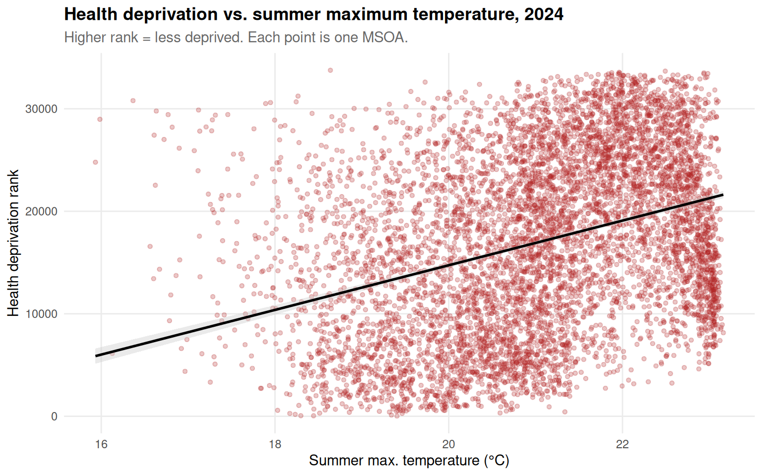
Both heat exposure measures are strongly and positively associated with the MSOA health rank. A 1°C increase in mean summer maximum temperature is associated with a shift of about 2,179 places up the national ranking, and one additional extreme hot day per year with a shift of about 2,485 places. Both coefficients are highly significant (p < 0.001).
In the English IMD convention, rank 1 is the most health-deprived area, so a positive coefficient means hotter MSOAs tend to rank as less health-deprived. This counterintuitive sign almost certainly reflects geography rather than a protective effect of heat: warmer parts of England (the south and southeast) are on average more affluent and healthier than cooler post-industrial areas in the north and midlands. The two specifications explain a similar share of variation (R² ≈ 0.12), with extreme hot days a marginally better fit.
These bivariate associations confound heat exposure with regional patterns of deprivation, age structure, urbanity, and housing.
A scatter plot for summer_max_tmp makes the relationship visible:
ggplot(msoa_2024, aes(x = summer_max_tmp, y = health_rank_msoa)) +
  geom_point(alpha = 0.25, size = 1.2, colour = "firebrick") +
  geom_smooth(method = "lm", se = TRUE,
              colour = "black", linewidth = 0.9, fill = "grey80") +
  labs(
    title    = "Health deprivation vs. summer maximum temperature, 2024",
    subtitle = "Higher rank = less deprived. Each point is one MSOA.",
    x = "Summer max. temperature (°C)",
    y = "Health deprivation rank"
  ) +
  theme_minimal(base_size = 11) +
  theme(
    plot.title    = element_text(face = "bold"),
    plot.subtitle = element_text(colour = "grey40"),
    panel.grid.minor = element_blank()
  )
fig, ax = plt.subplots(figsize=(8, 5))

x = msoa_2024["summer_max_tmp"]
y = msoa_2024["health_rank_msoa"]

ax.scatter(x, y, alpha=0.25, s=10, color="firebrick")
<matplotlib.collections.PathCollection object at 0x7f18e475d040>slope, intercept, r_value, p_value, _ = stats.linregress(x, y)
x_line = np.linspace(x.min(), x.max(), 100)
ax.plot(x_line, slope * x_line + intercept, color="black", linewidth=2)[<matplotlib.lines.Line2D object at 0x7f18e475fcb0>]ax.set_title("Health deprivation vs. summer maximum temperature, 2024",
fontweight="bold")Text(0.5, 1.0, 'Health deprivation vs. summer maximum temperature, 2024')ax.set_xlabel("Summer max. temperature (°C)")Text(0.5, 0, 'Summer max. temperature (°C)')ax.set_ylabel("Health deprivation rank")Text(0, 0.5, 'Health deprivation rank')ax.grid(True, alpha=0.3)
plt.tight_layout()
plt.show()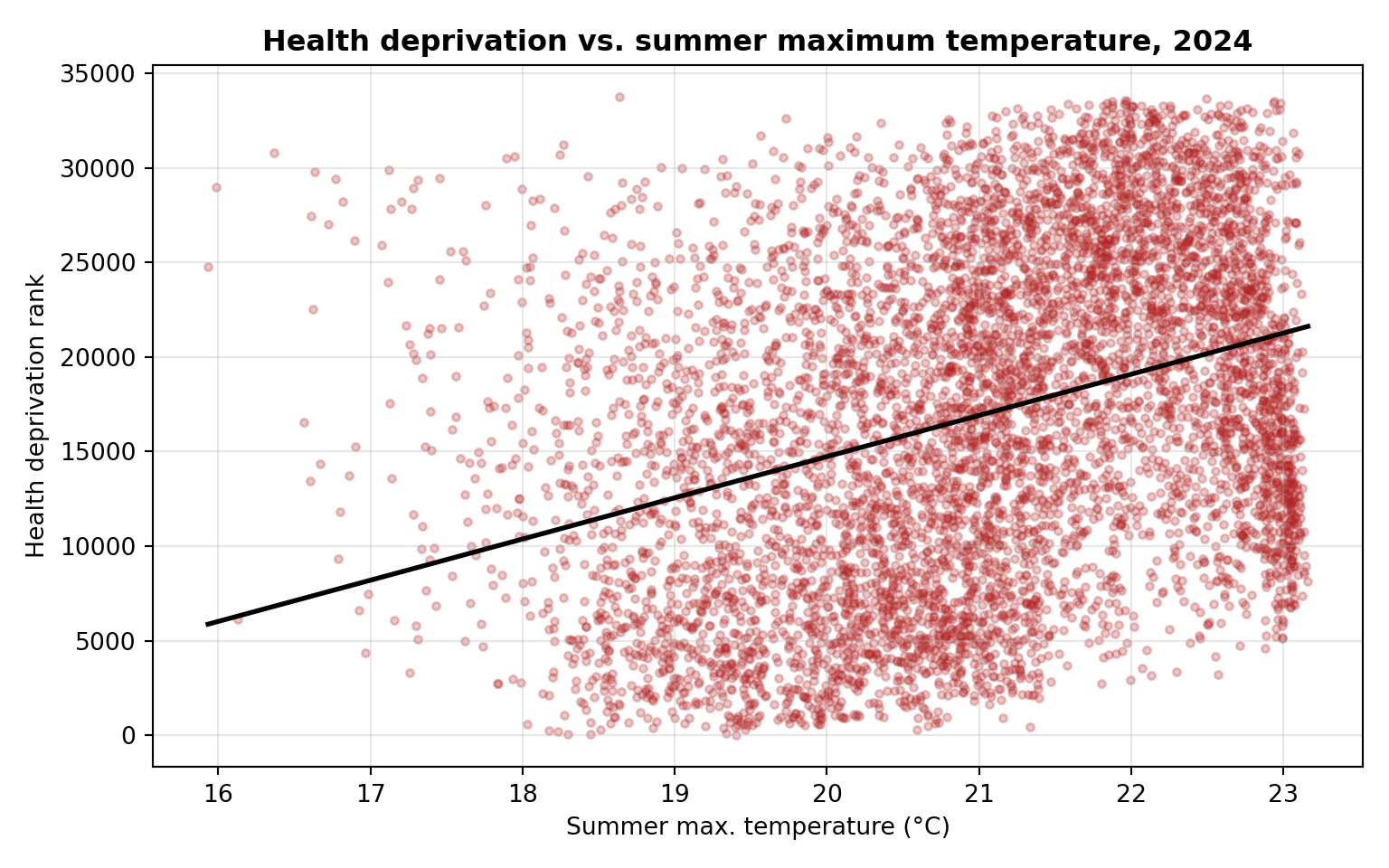
NoteWhat this regression can and cannot tell us
The slope coefficients tell us about the average association between heat exposure and deprivation in 2024. They do not tell us about causation: many factors influence both heat exposure and health outcomes, including:
- Socioeconomic and demographic composition: income, employment, education, age structure, ethnicity.
- Housing characteristics: building quality, insulation, heating systems, tenure, urban density.
- Environmental features: altitude, proximity to water, green space, urban heat island intensity.
- Health and vulnerability: prevalence of chronic illness, respiratory conditions.
- Infrastructure and access: public transport, energy affordability, healthcare access.
A serious causal analysis would require controlling for these — and even then, identifying a causal effect of heat exposure on health-related deprivation would need a research design (e.g. plausibly exogenous variation in heat exposure) that goes beyond a single cross-section.
Two questions a single cross-section cannot answer at all:
- Is the relationship stable over time, or has it strengthened or weakened?
- Has the gap between the most and least deprived MSOAs widened, narrowed, or held steady?
For both of these we need a panel.