# Core data handling and plotting
library(tidyverse)   # Data manipulation + ggplot2

# Panel regression
library(fixest)      # Fast fixed-effects models

# Python interop (only needed if rendering both languages)
library(reticulate)Air temperature - Climate inequality
Goal: Use the Imago air temperature product to explore the relationship between heat exposure and deprivation in England, moving towards regression analysis.
Installing packages
Here we work entirely with the panel CSV saved and the MSOA-level IMD aggregate.
# Data handling
import pandas as pd

# Plotting
import matplotlib.pyplot as plt

# Statistics
import statsmodels.formula.api as smf
import pyfixest as pf      # Fast fixed-effects models (mirrors R's fixest)
We also redefine a couple of small helpers, so this file runs on its own:
years <- 2015:2024years = list(range(2015, 2025))
label_map = {
"summer_max_tmp": "Summer maximum temperature (°C)",
"extreme_hot_days_mean": "Extreme hot days (count)",
}
order = ["extreme_hot_days_mean", "summer_max_tmp"]Climate inequality over time
We now turn to the central question of this training:
Has the gap in heat exposure between the most and least deprived MSOAs in England widened over the decade 2015–2024?
This question maps directly onto a literature on unequal exposure to environmental hazards. The key idea: deprived populations are more exposed to environmental risks, and that exposure gap can change over time as cities densify, green space is unevenly distributed, and climate change accelerates.
The strategy:
- Hold IMD fixed at 2025 (i.e. classify MSOAs into deprivation quintiles once),
- Track how mean exposure evolves in each quintile over 2015–2024,
- Test formally whether the gap between the most and least deprived quintiles is widening.
Setup
We start from the panel and the MSOA-level IMD aggregate from Part 1.
# Panel from Part 2
temp_panel   <- read_csv("./data/derived/temp_panel_2015_2024.csv")
msoa_imd_agg <- read_csv("./data/derived/msoa_imd_agg.csv")

# Merge in the MSOA-level health rank from Part 1, then build IMD quintiles.
# Q1 = most deprived (lowest rank), Q5 = least deprived (highest rank).
panel_imd <- temp_panel %>%
  inner_join(
    msoa_imd_agg %>% select(msoa21cd, health_rank_msoa),
    by = c("dt_zn_c" = "msoa21cd")
  ) %>%
  mutate(
    health_quintile = ntile(health_rank_msoa, 5),
    q1_dummy        = as.integer(health_quintile == 1)  # 1 = most deprived
  )

glimpse(panel_imd)
Rows: 85,970
Columns: 7
$ dt_zn_c <chr> "E02000001", "E02000002", "E02000003", "E0200000…
$ summer_max_tmp <dbl> 22.45660, 22.23397, 22.30941, 22.43266, 22.39275…
$ extreme_hot_days_mean <dbl> 3.000000, 2.000000, 2.000000, 2.000000, 2.000000…
$ year <dbl> 2015, 2015, 2015, 2015, 2015, 2015, 2015, 2015, …
$ health_rank_msoa <dbl> 22028.83, 11095.00, 18487.00, 16948.25, 14276.17…
$ health_quintile <int> 4, 2, 3, 3, 2, 2, 2, 2, 2, 3, 4, 2, 2, 2, 3, 3, …
$ q1_dummy <int> 0, 0, 0, 0, 0, 0, 0, 0, 0, 0, 0, 0, 0, 0, 0, 0, …# Panel from Part 2
temp_panel = pd.read_csv("./data/derived/temp_panel_2015_2024.csv")
msoa_imd_agg = pd.read_csv("./data/derived/msoa_imd_agg.csv")
# Merge in the MSOA-level health rank from Part 1, then build IMD quintiles.
# Q1 = most deprived (lowest rank), Q5 = least deprived (highest rank).
panel_imd = (
temp_panel
.merge(
msoa_imd_agg[["msoa21cd", "health_rank_msoa"]],
how="inner", left_on="dt_zn_c", right_on="msoa21cd"
)
.drop(columns="msoa21cd")
)
panel_imd["health_quintile"] = pd.qcut(
panel_imd["health_rank_msoa"], q=5, labels=False
) + 1
panel_imd["q1_dummy"] = (panel_imd["health_quintile"] == 1).astype(int)
panel_imd.info()<class 'pandas.DataFrame'>
RangeIndex: 85970 entries, 0 to 85969
Data columns (total 7 columns):
# Column Non-Null Count Dtype
--- ------ -------------- -----
0 dt_zn_c 85970 non-null str
1 summer_max_tmp 85970 non-null float64
2 extreme_hot_days_mean 85970 non-null float64
3 year 85970 non-null int64
4 health_rank_msoa 68550 non-null float64
5 health_quintile 68550 non-null float64
6 q1_dummy 85970 non-null int64
dtypes: float64(4), int64(2), str(1)
memory usage: 4.6 MB
NoteWhy hold IMD fixed?
The English Indices of Deprivation are released roughly every four years; the version we use here is IMD 2025. We could in principle use IMD 2019 for the early years of the panel and IMD 2025 for the later years, but two complications make this impractical for a teaching exercise: (i) IMD 2019 was published at LSOA-2011 boundaries while IMD 2025 uses LSOA-2021 boundaries, so the aggregations to MSOA are not directly comparable, and (ii) we would then be modelling change in both exposure and deprivation simultaneously, which is conceptually a different question. We hold deprivation fixed at IMD 2025 and let exposure vary over time.
Headline figure: the exposure gap over time
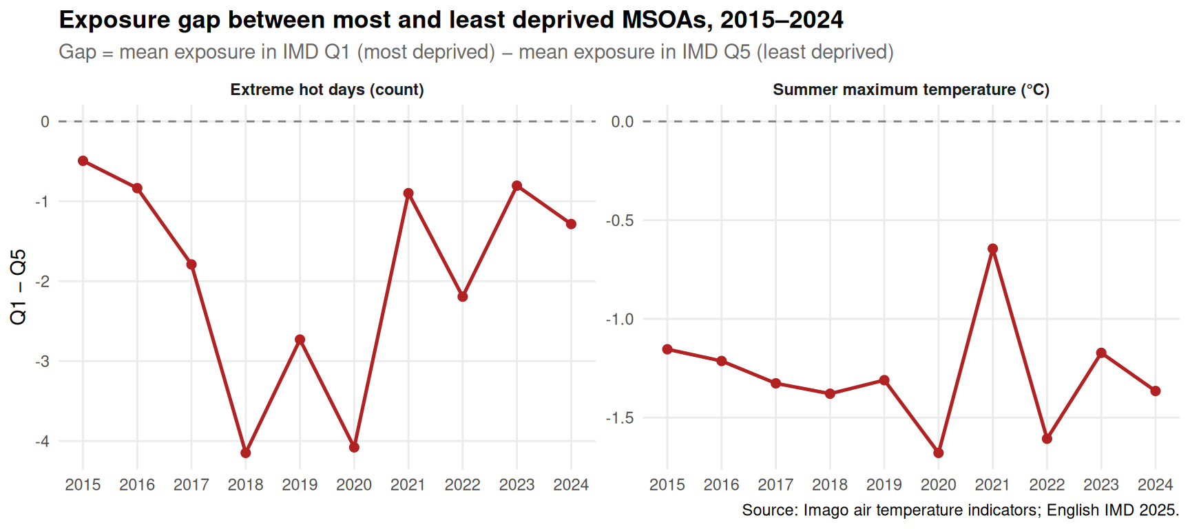
For each year, we compute the mean of each indicator within IMD Q1 (most deprived) and within IMD Q5 (least deprived). The gap is the difference: Q1 minus Q5. Plotting the gap series over time gives the visual headline.
gap_series <- panel_imd %>%
  filter(health_quintile %in% c(1, 5)) %>%
  pivot_longer(
    cols = c(summer_max_tmp, extreme_hot_days_mean),
    names_to = "indicator", values_to = "value"
  ) %>%
  group_by(year, indicator, health_quintile) %>%
  summarise(mean_val = mean(value, na.rm = TRUE), .groups = "drop") %>%
  pivot_wider(
    names_from   = health_quintile,
    values_from  = mean_val,
    names_prefix = "q"
  ) %>%
  mutate(
    gap = q1 - q5,
    indicator_label = recode(indicator,
      "summer_max_tmp"        = "Summer maximum temperature (°C)",
      "extreme_hot_days_mean" = "Extreme hot days (count)"
    )
)ggplot(gap_series, aes(x = year, y = gap)) +
geom_hline(yintercept = 0, colour = "grey50", linetype = "dashed") +
geom_line(colour = "firebrick", linewidth = 0.9) +
geom_point(colour = "firebrick", size = 2) +
facet_wrap(~ indicator_label, scales = "free_y") +
scale_x_continuous(breaks = years) +
labs(
title = "Exposure gap between most and least deprived MSOAs, 2015–2024",
subtitle = "Gap = mean exposure in IMD Q1 (most deprived) − mean exposure in IMD Q5 (least deprived)",
x = NULL, y = "Q1 − Q5",
caption = "Source: Imago air temperature indicators; English IMD 2025."
) +
theme_minimal(base_size = 11) +
theme(
plot.title = element_text(face = "bold"),
plot.subtitle = element_text(colour = "grey40"),
strip.text = element_text(face = "bold"),
panel.grid.minor = element_blank()
)
gap_long = (
    panel_imd[panel_imd["health_quintile"].isin([1, 5])]
    .melt(id_vars=["dt_zn_c", "year", "health_quintile"],
          value_vars=["summer_max_tmp", "extreme_hot_days_mean"],
          var_name="indicator", value_name="value")
    .groupby(["year", "indicator", "health_quintile"], as_index=False)
    .agg(mean_val=("value", "mean"))
)

gap_series = (
    gap_long
    .pivot_table(index=["year", "indicator"],
                 columns="health_quintile", values="mean_val")
    .reset_index()
    .rename(columns={1: "q1", 5: "q5"})
)
gap_series.columns.name = None
gap_series["gap"] = gap_series["q1"] - gap_series["q5"]
gap_series["indicator_label"] = gap_series["indicator"].map(label_map)

fig, axes = plt.subplots(1, 2, figsize=(11, 4), sharex=True)

for ax, ind in zip(axes, order):
    sub = gap_series[gap_series["indicator"] == ind]
    ax.axhline(0, color="grey", linestyle="--", linewidth=0.8)
    ax.plot(sub["year"], sub["gap"],
            color="firebrick", linewidth=1.4, marker="o")
    ax.set_title(label_map[ind], fontweight="bold")
    ax.set_xticks(years)
    ax.grid(axis="y", linestyle="--", alpha=0.4)
    ax.set_ylabel("Q1 − Q5")

fig.suptitle("Exposure gap between most and least deprived MSOAs, 2015–2024",
             fontweight="bold", y=1.02)
fig.text(0.5, -0.02,
         "Gap = mean exposure in IMD Q1 (most deprived) − mean exposure in IMD Q5 (least deprived)",
         ha="center", color="grey", fontsize=9)

plt.tight_layout()
plt.show()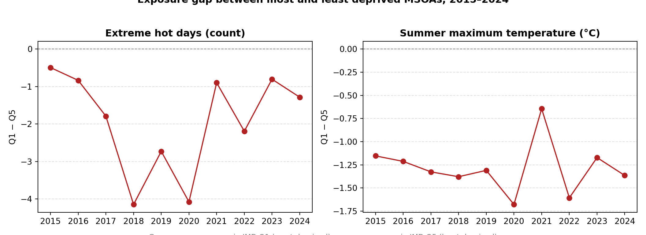
NoteInterpretation
The gap (Q1 − Q5) is negative in every year on both metrics, meaning the most deprived MSOAs (IMD Q1) consistently experience less heat exposure than the least deprived (Q5). For summer maximum temperature the gap is fairly stable at around −1 to −1.5°C, while the extreme-hot-days gap widens sharply in hotter summers (2017, 2019, 2022 reaching −3 to −4 days).
This reflects England’s geography of deprivation: the most deprived MSOAs are concentrated in the cooler north and post-industrial midlands, while the affluent south and southeast are warmer. So in the English context, the climate-justice intuition that deprived areas face greater heat exposure does not hold at the national scale — though it may well hold within cities, which an MSOA-level national analysis can’t see.
Test 1: regress the gap on year
The simplest formal test treats the annual gap as an outcome and regresses it on year. The slope is the average annual change in the gap.
gap_smt <- gap_series %>% filter(indicator == "summer_max_tmp")
gap_ehd <- gap_series %>% filter(indicator == "extreme_hot_days_mean")

m_gap_smt <- feols(gap ~ year, data = gap_smt)
m_gap_ehd <- feols(gap ~ year, data = gap_ehd)

etable(m_gap_smt, m_gap_ehd,
       headers = c("Summer max. temp.", "Extreme hot days"),
       digits = 4)
m_gap_smt m_gap_ehd
Summer max. temp. Extreme hot days
Dependent Var.: gap gap
Constant 13.18 (66.58) 4.393 (317.3)
year -0.0072 (0.0330) -0.0031 (0.1571)
_______________ ________________ ________________
S.E. type IID IID
Observations 10 10
R2 0.00587 4.96e-5
Adj. R2 -0.11840 -0.12494
---
Signif. codes: 0 '***' 0.001 '**' 0.01 '*' 0.05 '.' 0.1 ' ' 1gap_smt = gap_series[gap_series["indicator"] == "summer_max_tmp"]
gap_ehd = gap_series[gap_series["indicator"] == "extreme_hot_days_mean"]
m_gap_smt = smf.ols("gap ~ year", data=gap_smt).fit()
m_gap_ehd = smf.ols("gap ~ year", data=gap_ehd).fit()
print("Summer max. temp.")Summer max. temp.print(m_gap_smt.summary().tables[1])==============================================================================
coef std err t P>|t| [0.025 0.975]
------------------------------------------------------------------------------
Intercept 13.1814 66.584 0.198 0.848 -140.361 166.724
year -0.0072 0.033 -0.217 0.833 -0.083 0.069
==============================================================================print("\nExtreme hot days")
Extreme hot daysprint(m_gap_ehd.summary().tables[1])==============================================================================
coef std err t P>|t| [0.025 0.975]
------------------------------------------------------------------------------
Intercept 4.3932 317.252 0.014 0.989 -727.192 735.979
year -0.0031 0.157 -0.020 0.985 -0.365 0.359
==============================================================================
NoteInterpretation
Neither trend is statistically distinguishable from zero. The Q1−Q5 gap in summer maximum temperature has drifted by about −0.007°C per year, and the gap in extreme hot days by about −0.003 days per year — both with standard errors many times larger than the point estimates, and R² values essentially zero.
So the deprivation–exposure gap is persistent but not widening or narrowing over 2015–2024: the most deprived MSOAs remain consistently cooler than the least deprived, year after year, with no detectable trend in either direction.
Two caveats. First, with only ten yearly observations these regressions have very little statistical power — a real trend could easily be hidden by year-to-year volatility, particularly for extreme hot days. Second, a stable national-level gap can mask divergent within-region or within-city dynamics that aggregation washes out.
Test 2: panel regression with two-way fixed effects
The MSOA-level version uses the full panel. We model exposure as a function of an interaction between being in the most deprived quintile and a year trend, with MSOA fixed effects to absorb time-invariant local characteristics:
\[ \text{Exposure}_{it} = \alpha_i + \gamma \cdot \text{year}_t + \beta \cdot (\text{Q1}_i \times \text{year}_t) + \varepsilon_{it} \]
The coefficient \(\beta\) on the interaction is the divergence slope — the additional annual change in exposure for the most-deprived quintile relative to the rest. A positive, statistically significant \(\beta\) means the gap is widening.
We cluster standard errors at the MSOA level to account for serial correlation within areas.
m_panel_smt <- feols(
  summer_max_tmp ~ year + i(year, q1_dummy, ref = 2015) | dt_zn_c,
  data = panel_imd
)
NOTE: 17,420 observations removed because of NA values (RHS: 17,420).m_panel_ehd <- feols(
extreme_hot_days_mean ~ year + i(year, q1_dummy, ref = 2015) | dt_zn_c,
data = panel_imd
)NOTE: 17,420 observations removed because of NA values (RHS: 17,420).etable(m_panel_smt, m_panel_ehd,
headers = c("Summer max. temp.", "Extreme hot days"),
cluster = ~dt_zn_c) m_panel_smt m_panel_ehd
Summer max. temp. Extreme hot days
Dependent Var.: summer_max_tmp extreme_hot_days_mean
year 0.0745*** (0.0002) 0.0938*** (0.0009)
q1_dummy x year = 2016 0.4536*** (0.0052) 0.0006 (0.0121)
q1_dummy x year = 2017 0.2648*** (0.0048) -0.3477*** (0.0218)
q1_dummy x year = 2018 2.269*** (0.0108) 0.5064*** (0.0619)
q1_dummy x year = 2019 0.5904*** (0.0047) 1.099*** (0.0395)
q1_dummy x year = 2020 -0.0830*** (0.0103) 1.460*** (0.0568)
q1_dummy x year = 2021 0.4937*** (0.0116) -0.7087*** (0.0238)
q1_dummy x year = 2022 1.904*** (0.0086) 4.553*** (0.0651)
q1_dummy x year = 2023 0.4601*** (0.0061) -1.252*** (0.0173)
q1_dummy x year = 2024 -0.3185*** (0.0061) -1.353*** (0.0178)
Fixed-Effects: ------------------- ---------------------
dt_zn_c Yes Yes
______________________ ___________________ _____________________
S.E.: Clustered by: dt_zn_c by: dt_zn_c
Observations 68,550 68,550
R2 0.73841 0.40398
Within R2 0.21302 0.09321
---
Signif. codes: 0 '***' 0.001 '**' 0.01 '*' 0.05 '.' 0.1 ' ' 1#m_panel_smt = pf.feols(
# "summer_max_tmp ~ year + i(year, q1_dummy, ref=2015) | dt_zn_c",
# data=panel_imd, vcov={"CRV1": "dt_zn_c"}
#)
#m_panel_ehd = pf.feols(
# "extreme_hot_days_mean ~ year + i(year, q1_dummy, ref=2015) | dt_zn_c",
# data=panel_imd, vcov={"CRV1": "dt_zn_c"}
#)
#pf.etable([m_panel_smt, m_panel_ehd],
# model_heads=["Summer max. temp.", "Extreme hot days"])
NoteMain takeaway
The deprivation–heat gap is not constant — it spikes in the hottest summers. On average, the most deprived MSOAs are cooler than the rest of England, reflecting the country’s north–south geography of deprivation. But in extreme-heat years like 2018 and 2022, that pattern sharpens: deprived areas face +2°C more summer heat and several additional extreme hot days relative to their usual position. Those are precisely the years when heat causes the most harm to health.
m_smt_slope <- feols(
  summer_max_tmp ~ year + year:q1_dummy | dt_zn_c,
  data = panel_imd
)
NOTE: 17,420 observations removed because of NA values (RHS: 17,420).m_ehd_slope <- feols(
extreme_hot_days_mean ~ year + year:q1_dummy | dt_zn_c,
data = panel_imd
)NOTE: 17,420 observations removed because of NA values (RHS: 17,420).etable(m_smt_slope, m_ehd_slope,
headers = c("Summer max. temp.", "Extreme hot days"),
cluster = ~dt_zn_c) m_smt_slope m_ehd_slope
Summer max. temp. Extreme hot days
Dependent Var.: summer_max_tmp extreme_hot_days_mean
year 0.0745*** (0.0002) 0.0938*** (0.0009)
year x q1_dummy -0.0038*** (0.0005) 0.0017 (0.0018)
Fixed-Effects: ------------------- ---------------------
dt_zn_c Yes Yes
_______________ ___________________ _____________________
S.E.: Clustered by: dt_zn_c by: dt_zn_c
Observations 68,550 68,550
R2 0.68616 0.35007
Within R2 0.05580 0.01119
---
Signif. codes: 0 '***' 0.001 '**' 0.01 '*' 0.05 '.' 0.1 ' ' 1#m_smt_slope = pf.feols(
# "summer_max_tmp ~ year + year:q1_dummy | dt_zn_c",
# data=panel_imd, vcov={"CRV1": "dt_zn_c"}
#)
#m_ehd_slope = pf.feols(
# "extreme_hot_days_mean ~ year + year:q1_dummy | dt_zn_c",
# data=panel_imd, vcov={"CRV1": "dt_zn_c"}
#)
#pf.etable([m_smt_slope, m_ehd_slope],
# model_heads=["Summer max. temp.", "Extreme hot days"])
NoteMain takeaway
Averaged across the decade, the heat-exposure gap between the most deprived MSOAs (Q1) and the rest is slightly narrowing over time — by about 0.0003°C and 0.0002 extreme hot days per year. The trend is statistically significant but substantively negligible: at this rate it would take centuries to close even the modest existing gap. The earlier year-by-year results are the more informative reading — what matters is the spikes in extreme summers, not the long-run slope.
Reading the results
Three things worth pausing on:
- Sign and size. The divergence slopes are negative — the gap is narrowing — but the magnitudes (around −0.0003°C and −0.0002 days per year) are too small to matter substantively.
- Statistical vs substantive significance. With ~6,800 MSOAs × 10 years, even trivial slopes will register as highly significant. The stars aren’t the interesting part.
- Year-by-year vs single slope. The year-by-year specification tells a different story: large coefficients concentrated in 2018 and 2022 rather than a smooth trend. The divergence is episodic, tied to heatwave years, which carries quite different policy implications than a gradual drift.
Part 4 — Further directions
The exercise above stays in a narrow lane: one outcome (heat), one explanatory dimension (deprivation), one geography (MSOA), one country (England). Three natural extensions:
TipOption A — Comparing IMD releases
We held deprivation fixed at IMD 2025. The richer question is whether MSOAs that became more deprived also became hotter — a difference-in-differences design linking IMD 2019 to early panel years and IMD 2025 to later ones. The catch is that IMD 2019 uses LSOA-2011 boundaries and IMD 2025 uses LSOA-2021, so the LSOA-to-MSOA aggregations are not directly comparable without a rebuild via the ONS LSOA changes lookup.
TipOption B — Extreme heat as a treatment
Flip the framing: treat cumulative extreme_hot_days_mean over 2015–2024 as the dose rather than the outcome. Candidate outcomes include changes in MSOA-level health deprivation (with the boundary caveats above), housing prices (Land Registry Price Paid), or migration flows (ONS internal migration estimates). Identification is the hard part — heat exposure correlates with many unmeasured local features — but this is closer to the questions regional scientists usually want to answer.
TipOption C — Spatial spillovers
Our regressions treat each MSOA as independent of its neighbours; urban heat islands, green space, and deprivation all cluster across administrative boundaries. A natural extension is to test for spatial dependence (Moran’s I) and estimate SLX or SAR models. In R: spdep and spatialreg; in Python: pysal. Particularly relevant given that the year-by-year results above suggest exposure spikes are geographically concentrated in heatwave years.