# Geospatial Libraries
import geopandas as gpd
import numpy as np

# Plotting
import matplotlib.pyplot as pltPrecipitation - Seasonal Patterns
Goal: Using the Imago MSOA Precipitation Product, explore how rainfall changes across the seasons and identify which seasons contribute most to annual rainfall across different parts of the UK.
Data:
A question for the data
In the first case study, we mapped how rainfall was distributed across the UK. However, annual totals alone do not tell the whole story, as they hide the seasonal patterns behind those figures.
A local authority experiencing a particularly wet year may have received consistently high rainfall throughout the year, or it may have been heavily influenced by a single unusually wet season.
To investigate this, we break annual rainfall into winter, spring, summer, and autumn totals and examine how seasonal rainfall patterns vary across the country.
Installing Libraries
Loading the Data
Using geopandas, we can read the gpkg. As it’s a gpkg it already has the boundaries and will not need a separate boundary file.
precip_msoa = gpd.read_file("data/precipitation_indicators_MSOA_2024.gpkg")
precip_msoa.head()| dt_zn_c | dt_zn_n | rainfall_annual_mm | winter_rainfall | spring_rainfall | summer_rainfall | autumn_rainfall | annual_anomaly_abs | annual_anomaly_std | extreme_days_4sd | year | geometry | |
|---|---|---|---|---|---|---|---|---|---|---|---|---|
| 0 | E02000001 | City of London 001 | 696.647095 | 223.671677 | 189.220276 | 107.580292 | 218.248856 | 158.290131 | 2.148560 | 26.304880 | 2024 | MULTIPOLYGON (((532135.138 182198.131, 532158.... |
| 1 | E02000002 | Barking and Dagenham 001 | 695.338257 | 236.243835 | 192.781601 | 106.833694 | 205.600983 | 131.554367 | 1.715453 | 23.520077 | 2024 | MULTIPOLYGON (((548881.563 190845.265, 548881.... |
| 2 | E02000003 | Barking and Dagenham 002 | 667.498779 | 230.828064 | 185.345505 | 100.507462 | 195.728653 | 120.716499 | 1.595210 | 22.027685 | 2024 | MULTIPOLYGON (((549102.438 189324.625, 548954.... |
| 3 | E02000004 | Barking and Dagenham 003 | 611.439758 | 218.056824 | 171.161316 | 89.372581 | 175.921600 | 93.010658 | 1.238803 | 23.146259 | 2024 | MULTIPOLYGON (((551550.056 187364.705, 551478 ... |
| 4 | E02000005 | Barking and Dagenham 004 | 632.301819 | 224.054337 | 176.073090 | 93.059616 | 183.112747 | 102.117798 | 1.371893 | 22.568747 | 2024 | MULTIPOLYGON (((549099.634 187656.076, 549161.... |
This file contains multiple rainfall indicators. For this notebook, we are using the four seasonal indicators, which follow meteorological seasons:
winter_rainfall: Mean rainfall in millimeters during the winter season (December to February)spring_rainfall: Mean rainfall in millimeters during the spring season (March to May)summer_rainfall: Mean rainfall in millimeters during the summer season (June to August)autumn_rainfall: Mean rainfall in millimeters during the autumn season (September to November)
Understanding Seasonal Rainfall
seasonal_cols = [
    "winter_rainfall",
    "spring_rainfall",
    "summer_rainfall",
    "autumn_rainfall",
]

precip_msoa[seasonal_cols].agg(["mean", "std", "min", "max"])| winter_rainfall | spring_rainfall | summer_rainfall | autumn_rainfall | |
|---|---|---|---|---|
| mean | 337.598752 | 256.169848 | 166.399425 | 272.438569 |
| std | 118.987462 | 66.683888 | 69.266426 | 88.646086 |
| min | 175.249985 | 130.992889 | 64.361282 | 103.140388 |
| max | 1324.960449 | 775.110901 | 807.014648 | 805.231628 |
Note
As expected, winter receives the highest average rainfall while summer receives the lowest. This reflects the UK’s temperate maritime climate, where rainfall generally increases through autumn into winter before declining again through spring and summer. Interestingly, the maximum rainfall recorded in summer exceeds that of both spring and autumn. Mapping these data will help us examine whether the UK is universally dominated by winter rainfall, or if there is significant regional variation in seasonal patterns.
Comparing Seasonal Rainfall
Summary statistics provide a useful overview of each season, but they do not clearly show how rainfall varies between them. A box plot allows us to compare the median rainfall, the spread of values, and the overall variability across all four seasons at the same time.
season_cols = [
    "winter_rainfall",
    "spring_rainfall",
    "summer_rainfall",
    "autumn_rainfall",
]

fig, ax = plt.subplots(figsize=(8, 5))

precip_msoa[season_cols].boxplot(
    ax=ax,
    showfliers=False,
    patch_artist=True,
)

ax.set_title("Seasonal Rainfall Variability Across MSOAs, 2024", fontweight="bold")
ax.set_ylabel("Rainfall (mm)")
ax.set_xlabel("")

ax.grid(axis="y", linestyle="--", alpha=0.3)
ax.grid(axis="x", visible=False)

plt.tight_layout()
plt.show()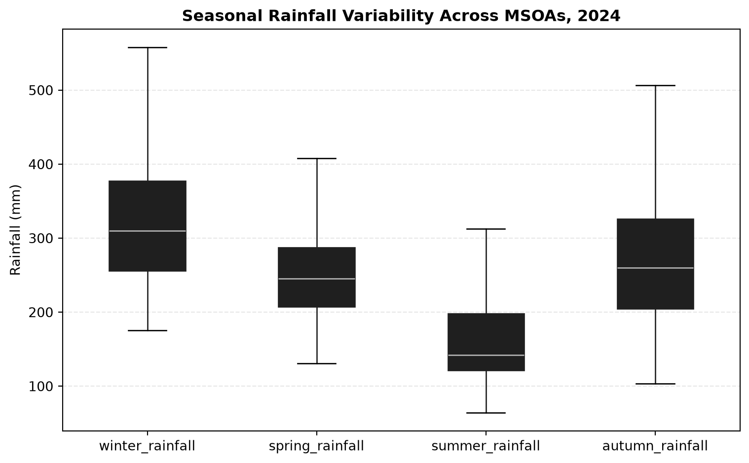
NotePatterns
The box plots show that rainfall varies substantially between seasons. Winter has the highest median rainfall and also the widest spread of values, indicating that many of the wettest MSOAs receive particularly large amounts of winter rainfall. Autumn also shows considerable variability, while spring has a more moderate spread. Summer has the lowest median rainfall and the smallest interquartile range, suggesting that rainfall totals are generally lower and more consistent across much of the UK during this season.
All four seasons contain values well above the upper quartile, indicating that some locations consistently receive much more rainfall than the majority of MSOAs regardless of season. This suggests that regional geography continues to influence rainfall throughout the year.
While this comparison tells us how rainfall varies statistically between the seasons, it does not show where these differences occur. To understand the geographical patterns behind these statistics, we next map rainfall for each season individually.
Visualising Seasonal Rainfall
The most intuitive way to see the seasonal affects across the year in the UK is through mapping each individual season. It allows us to identify how rainfall patterns change through the year and whether annual rainfall totals are driven by the same seasons across the country.
season_cols = {
    "winter_rainfall": "Winter",
    "spring_rainfall": "Spring",
    "summer_rainfall": "Summer",
    "autumn_rainfall": "Autumn",
}

fig, axes = plt.subplots(2, 2, figsize=(12, 10))

for ax, (col, season) in zip(axes.flatten(), season_cols.items()):
    p01 = precip_msoa[col].quantile(0.01)
    p99 = precip_msoa[col].quantile(0.99)

    precip_msoa.plot(
        column=col,
        cmap="Blues",
        legend=True,
        ax=ax,
        vmin=p01,
        vmax=p99,
        linewidth=0,
    )

    ax.set_title(f"{season} Rainfall")
    ax.set_axis_off()

fig.suptitle("Seasonal Rainfall Across UK MSOAs, 2024", fontweight="bold")
plt.tight_layout()
plt.show()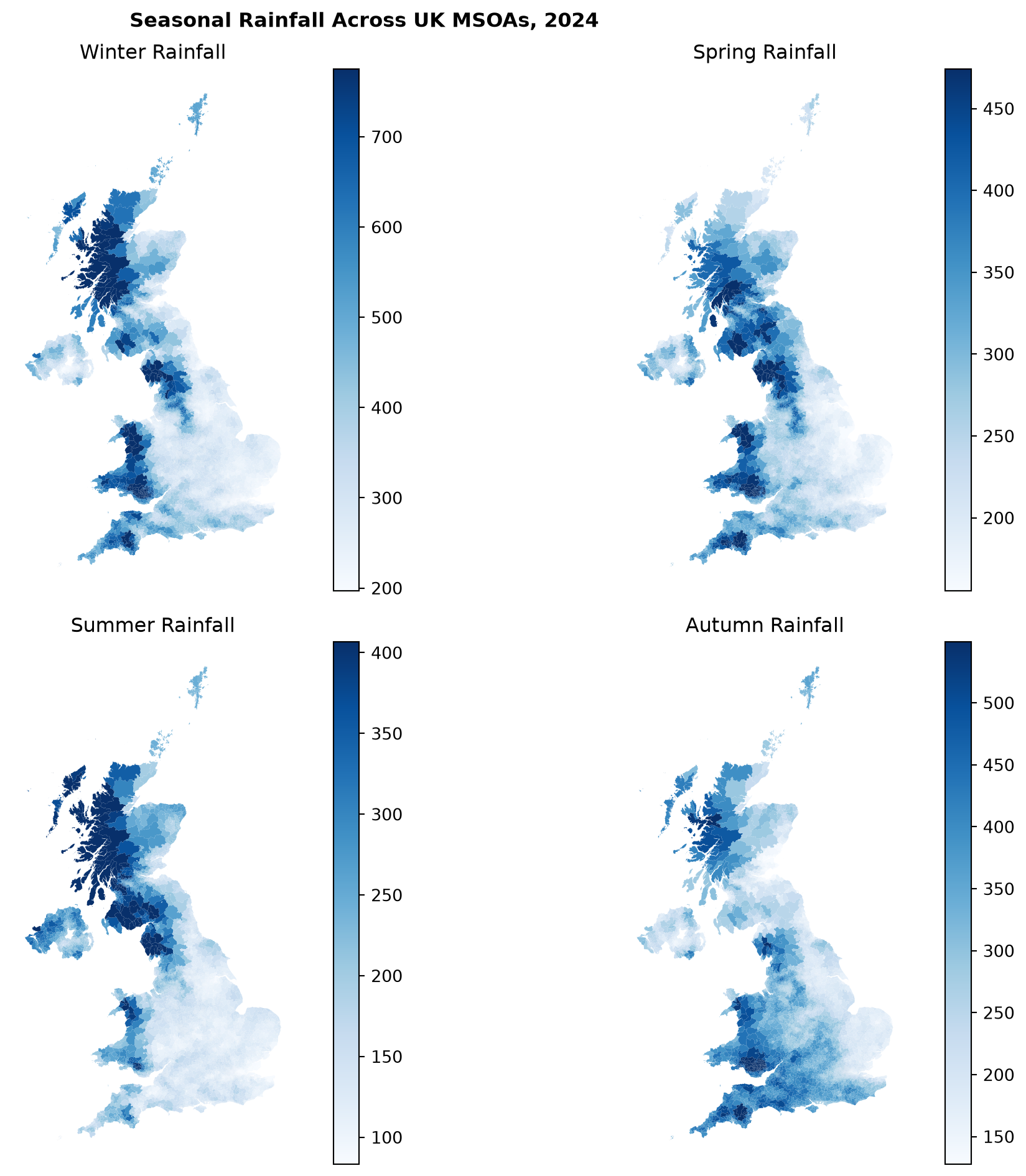
Note
We can clearly see that each season is spatially very unique. Most notably, summer rainfall is highly concentrated, with Scotland, northern England, and Wales receiving the highest rainfall totals while the rest of the country, especially southern and eastern England, receives relatively little. In contrast, autumn rainfall is far more evenly distributed across the country.
Although the general pattern of a wetter northwest and drier southeast holds true, a season-by-season view shows that the divide is primarily a west-east split. We can see that one of the rainiest parts of the country across all seasons is Cumbria.
Contribution of each season to total rainfall
The maps above show where rainfall occurs during each season, but they do not tell us how important each season is to the UK’s overall rainfall total. A season may have a distinctive spatial pattern while still contributing relatively little to the annual rainfall received across the country.
To understand which seasons had the greatest influence on annual rainfall in 2024, we calculate the proportion of total rainfall contributed by winter, spring, summer, and autumn across all MSOAs.
season_cols = [
    "winter_rainfall",
    "spring_rainfall",
    "summer_rainfall",
    "autumn_rainfall",
]

season_totals = precip_msoa[season_cols].sum()

season_percent = (season_totals / season_totals.sum()) * 100
print(f"{round(season_percent, 0)}")

fig, ax = plt.subplots(figsize=(7, 5))

season_percent.plot(kind="bar", color="darkslategrey", edgecolor="black", ax=ax)

ax.set_ylabel("Contribution to annual rainfall (%)")
ax.set_xlabel("")
ax.set_title("Seasonal Contribution to UK Rainfall, 2024", fontweight="bold")
ax.grid(axis="y", linestyle="--", alpha=0.3)
ax.grid(axis="x", visible=False)

plt.tight_layout()
plt.show()
winter_rainfall 33.0
spring_rainfall 25.0
summer_rainfall 16.0
autumn_rainfall 26.0
dtype: float64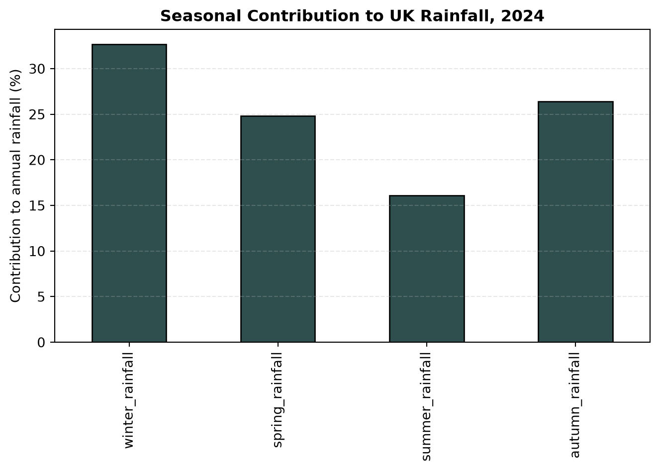
At a national level, rainfall is not distributed evenly throughout the year. Some seasons contribute a substantially larger share of annual rainfall than others.
Winter contributes the largest proportion of rainfall across the UK, followed by autumn, while summer contributes the smallest share. This helps explain why annual rainfall patterns often resemble the winter rainfall map more closely than the summer rainfall map.
However, national averages can hide substantial regional variation. A season that contributes relatively little rainfall nationally may still be the dominant rainfall season in particular parts of the country.
To explore this local variation, we identify the season that contributes the most rainfall to each MSOA and map the dominant rainfall season across the UK.
import pandas as pd
import matplotlib.colors as mcolors

# Map raw column names to clean, readable names for the legend
season_display_names = {
    "winter_rainfall": "Winter",
    "spring_rainfall": "Spring",
    "summer_rainfall": "Summer",
    "autumn_rainfall": "Autumn",
}
precip_msoa["dominant_season_name"] = precip_msoa[season_cols].idxmax(axis=1).map(season_display_names)

# Order categories so they display in a logical seasonal flow in the legend
precip_msoa["dominant_season_name"] = pd.Categorical(
    precip_msoa["dominant_season_name"],
    categories=["Winter", "Spring", "Summer", "Autumn"],
    ordered=True,
)

# Nordic Frost color palette (Summer modified to soft beige):
# Winter = Midnight Blue, Spring = Ice Blue, Summer = Soft Beige, Autumn = Steel Blue
colors_nordic = ["#2c3e50", "#a8dadc", "#e8d7c3", "#457b9d"]
cmap_seasons = mcolors.ListedColormap(colors_nordic)

fig, ax = plt.subplots(figsize=(7, 9))

precip_msoa.plot(
    column="dominant_season_name",
    categorical=True,
    legend=True,
    ax=ax,
    cmap=cmap_seasons,
)

ax.set_title("Dominant Rainfall Season by MSOA", fontweight="bold")
ax.axis("off")
plt.show()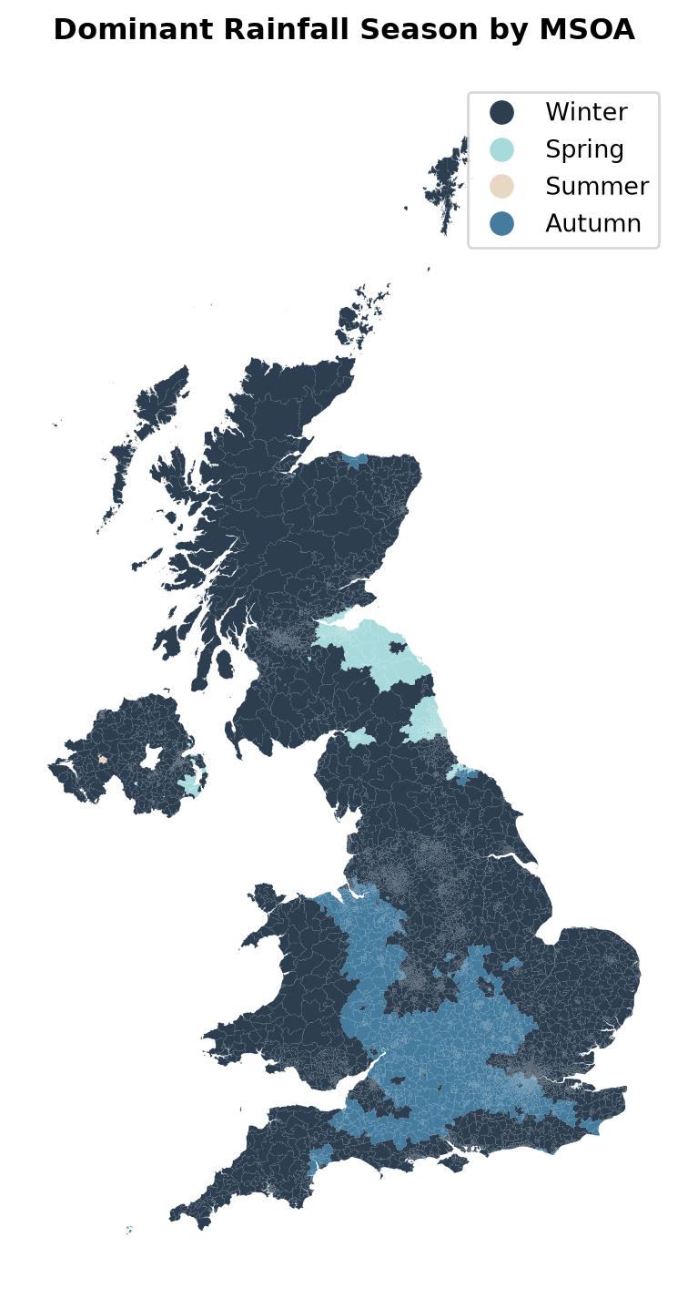
Note
The dominant season map simplifies the four seasonal rainfall maps into a single question: which season contributes the most rainfall to each MSOA?
Winter dominates annual rainfall across Scotland, Wales, Northern Ireland, and most of England. However, autumn is the leading contributor in many MSOAs across southern England and along the Welsh border.
Spring dominance is limited to County Down and the Northumberland-Scotland border, while summer is the dominant season in just a single MSOA in County Tyrone. Consequently, summer rainfall, though sometimes extreme, rarely drives annual totals.
What have we learnt?
- Rainfall distributions differ between seasons.
- Seasonal rainfall patterns vary geographically across the UK.
- Winter is the dominant rainfall season across most of the country.
- Southern England is more strongly influenced by autumn rainfall than many northern and western regions.
- Areas with similar annual rainfall totals may reach those totals through very different seasonal patterns.
Understanding these seasonal drivers provides important context when interpreting annual rainfall statistics. A wet year is not necessarily the result of consistently high rainfall throughout the year, it may have instead be driven by one particularly influential season.
In the next case study, we move beyond rainfall totals and investigate whether the wettest places were also the most unusual by comparing annual rainfall against long term norms.